In the previous examples we have essentially ignored time by defining models that map inputs to outputs in a single forward pass (e.g., we configured the default synapse to be None). In this example we’ll introduce a simple process model of information retrieval based on this standard Nengo tutorial. The idea is similar to this example where
we encoded role/filler information using semantic pointers and then retrieved a cued attribute. But in this example, rather than presenting the whole trace at once, we will present the input Role/Filler pairs one at a time and have the network remember them. Once all the bound pairs have been added to the memory, we can then query the model with a cue to test retrieval accuracy.
[1]:
%matplotlib inline

from functools import partial
import itertools
from urllib.request import urlretrieve
import zipfile

import matplotlib.pyplot as plt
import nengo
import nengo.spa as spa
import nengo_dl
import numpy as np
import tensorflow as tf
First we’ll define a function for generating training data. Note that this function will produce arrays of shape (n_inputs, n_steps, dims), where n_steps will be the number of time steps in the process we want to model. To start, we’ll generate simple examples in which the input trajectory consists of a single semantic pointer presented for some number of time steps, and the desired output trajectory involves maintaining a representation of that semantic pointer for some further number
of time steps.
[2]:
def get_memory_data(n_inputs, dims, seed, t_int, t_mem, dt=0.001):
    int_steps = int(t_int / dt)
    mem_steps = int(t_mem / dt)
    n_steps = int_steps + mem_steps

    rng = np.random.RandomState(seed)
    vocab = spa.Vocabulary(dimensions=dims, rng=rng, max_similarity=1)

    # initialize arrays for input and output trajectories
    inputs = np.zeros((n_inputs, n_steps, dims))
    outputs = np.zeros((n_inputs, n_steps, dims))

    # iterate through examples to be generated, fill arrays
    for n in range(n_inputs):
        name = "SP_%d" % n
        vocab.add(name, vocab.create_pointer())

        # create inputs and target memory for first pair
        inputs[n, :int_steps, :] = vocab[name].v
        outputs[n, :, :] = vocab[name].v

    # make scaling ramp for target output trajectories
    ramp = np.asarray([t / int_steps for t in range(int_steps)])
    ramp = np.concatenate((ramp, np.ones(n_steps - int_steps)))
    outputs = outputs * ramp[None, :, None]

    return inputs, outputs, vocab
Our first model will consist of a single input node and single recurrently connected memory ensemble. The input will present the input semantic pointer for a brief period, and then the task of the model will be to remember that semantic pointer over time.
[3]:
seed = 0
t_int = 0.01  # length of time for input presentation
t_mem = 0.04  # length of time for the network to store the input
dims = 32  # dimensionality of semantic pointer vectors
n_neurons = 5 * dims  # number of neurons for memory ensemble
minibatch_size = 32

with nengo.Network(seed=seed) as net:
    net.config[nengo.Ensemble].neuron_type = nengo.RectifiedLinear()
    net.config[nengo.Ensemble].gain = nengo.dists.Choice([1])
    net.config[nengo.Ensemble].bias = nengo.dists.Choice([0])

    sp_input = nengo.Node(np.zeros(dims))
    memory = nengo.Ensemble(n_neurons, dims)

    tau = 0.01  # synaptic time constant on recurrent connection
    nengo.Connection(sp_input, memory, transform=tau / t_int,
                     synapse=tau)
    nengo.Connection(memory, memory, transform=1, synapse=tau)

    sp_probe = nengo.Probe(sp_input)
    memory_probe = nengo.Probe(memory)
Next, we’ll run the model for the specified length of time in order to see how well the memory works.
[4]:
# generate test data
test_inputs, test_targets, test_vocab = get_memory_data(
    minibatch_size, dims, seed, t_int, t_mem)

# run with one example input
with nengo_dl.Simulator(
        net, seed=seed, minibatch_size=minibatch_size) as sim:
    sim.run(t_int+t_mem, data={sp_input: test_inputs})
Build finished in 0:00:00
Optimization finished in 0:00:00
|           Constructing graph: building inputs (0%)           | ETA:  --:--:--
/home/travis/build/nengo/nengo-dl/nengo_dl/simulator.py:131: UserWarning: No GPU support detected. It is recommended that you install tensorflow-gpu (`pip install tensorflow-gpu`).
  "No GPU support detected. It is recommended that you "
Construction finished in 0:00:00
Simulation finished in 0:00:00
[5]:
def plot_memory_example(sim, vocab, example_input=0):
    plt.figure(figsize=(8, 8))

    name = "SP_%d" % example_input

    plt.subplot(3, 1, 1)
    plt.plot(sim.trange(), nengo.spa.similarity(
        test_inputs[example_input], vocab), color="black", alpha=0.2)
    plt.plot(sim.trange(), nengo.spa.similarity(
        test_inputs[example_input], vocab[name].v), label=name)
    plt.legend(fontsize='x-small', loc='right')
    plt.ylim([-0.2, 1.1])
    plt.ylabel("Input")

    plt.subplot(3, 1, 2)
    plt.plot(sim.trange(), nengo.spa.similarity(
        test_targets[example_input], vocab), color="black", alpha=0.2)
    plt.plot(sim.trange(), nengo.spa.similarity(
        test_targets[example_input], vocab[name].v), label=name)
    plt.legend(fontsize='x-small', loc='right')
    plt.ylim([-0.2, 1.1])
    plt.ylabel("Target Memory")

    plt.subplot(3, 1, 3)
    plt.plot(
        sim.trange(), nengo.spa.similarity(
            sim.data[memory_probe][example_input], vocab),
        color="black", alpha=0.2)
    plt.plot(
        sim.trange(), nengo.spa.similarity(
            sim.data[memory_probe][example_input], vocab[name].v),
        label=name)
    plt.legend(fontsize='x-small', loc='right')
    plt.ylim([-0.2, 1.1])
    plt.ylabel("Output Memory")
    plt.xlabel("time [s]")

plot_memory_example(sim, test_vocab)
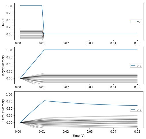
These plots show the similarity of the input/target/output vectors to all the items in the vocabulary. The similarity to the correct vocabulary item is highlighted, and we can see that while the memory is storing the correct item, that storage is not particularly stable.
To improve retention we can use Nengo DL to fine tune the model parameters. Training on temporally extended trajectories can be slow, so we’ll download pretrained parameters by default. You can train your own parameters by setting do_training=True (allowing you to vary things like learning rate or the number of training epochs to see the impact of those hyperparameters).
[6]:
do_training = False
if do_training:
    optimizer = tf.train.RMSPropOptimizer(1e-4)
    train_inputs, train_targets, _ = get_memory_data(
        4000, dims, seed, t_int, t_mem)

    with nengo_dl.Simulator(
            net, minibatch_size=minibatch_size, seed=seed) as sim:
        print('Test loss before: ', sim.loss(
            {sp_input: test_inputs, memory_probe: test_targets},
            {memory_probe: nengo_dl.obj.mse}))
        sim.train({sp_input: train_inputs, memory_probe: train_targets},
                  optimizer, n_epochs=100)
        print('Test loss after: ', sim.loss(
            {sp_input: test_inputs, memory_probe: test_targets},
            {memory_probe: nengo_dl.obj.mse}))

        sim.save_params('./mem_params')
else:
    # download pretrained parameters
    urlretrieve(
        "https://drive.google.com/uc?export=download&id=1duAA6-NzKM4o7NhTVGwjGp4GaKDIGO_g",
        "mem_params.zip")
    with zipfile.ZipFile("mem_params.zip") as f:
        f.extractall()
[7]:
with nengo_dl.Simulator(
        net, seed=seed, minibatch_size=minibatch_size) as sim:
    sim.load_params('./mem_params')
    sim.run(t_int+t_mem, data={sp_input: test_inputs})

plot_memory_example(sim, test_vocab)
Build finished in 0:00:00
Optimization finished in 0:00:00
Construction finished in 0:00:00
Simulation finished in 0:00:00
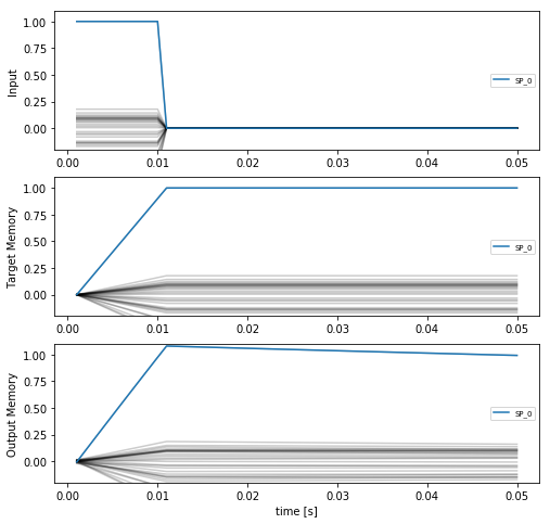
We can see that the training procedure significantly improves the stability of the memory.
Now we will return to the cued role/filler retrieval task from this example, and we will modify that task to include a memory aspect. Rather than presenting the complete trace as input all at once, we will present each \(ROLE\)/\(FILLER\) pair one at a time. The task of the network will be to bind each individual pair together, add them together to generate the full trace, store that trace in memory, and then when given one of the Roles as a cue, output the corresponding Filler. For example, one pass through the task would consist of the following phases:
| phase | role input | filler input | cue | target output |
|---|---|---|---|---|
| 1 | \(ROLE_0\) | \(FILLER_0\) | ||
| 2 | \(ROLE_1\) | \(FILLER_1\) | ||
| … | … | … | … | … |
| \(n\) | \(ROLE_n\) | \(FILLER_n\) | ||
| \(n+1\) | \(ROLE_x\) | \(FILLER_x\) |
First we will create a function to generate the input/target data for this task.
[8]:
def get_binding_data(n_inputs, n_pairs, dims, seed, t_int, t_mem,
                     dt=0.001):
    int_steps = int(t_int / dt)
    mem_steps = int(t_mem / dt)
    n_steps = int_steps*n_pairs + mem_steps

    rng = np.random.RandomState(seed)
    vocab = spa.Vocabulary(dimensions=dims, rng=rng, max_similarity=1)

    # initialize arrays for input and output trajectories
    roles = np.zeros((n_inputs, n_steps, dims))
    fills = np.zeros((n_inputs, n_steps, dims))
    cues = np.zeros((n_inputs, n_steps, dims))
    binding = np.zeros((n_inputs, n_steps, dims))
    memory = np.zeros((n_inputs, n_steps, dims))
    output = np.zeros((n_inputs, n_steps, dims))

    # iterate through examples to be generated, fill arrays
    for n in range(n_inputs):
        role_names = ["ROLE_%d_%d" % (n, i) for i in range(n_pairs)]
        filler_names = ["FILLER_%d_%d" % (n, i) for i in range(n_pairs)]

        # each role/filler pair is presented for t_int seconds
        for i in range(n_pairs):
            roles[n, i*int_steps:(i+1)*int_steps] = vocab.parse(
                role_names[i]).v
            fills[n, i*int_steps:(i+1)*int_steps] = vocab.parse(
                filler_names[i]).v
            binding[n, i*int_steps:(i+1)*int_steps] = vocab.parse(
                "%s*%s" % (role_names[i], filler_names[i])).v

        # randomly select a cue
        cue_idx = rng.randint(n_pairs)

        # cue is presented during the memorization period
        cues[n, -mem_steps:, :] = vocab[role_names[cue_idx]].v

        # the goal is to output the associated filler during the
        # memorization phase
        # note: we use nan for the target prior to the memorization
        # phase, to indicate that it doesn't matter what the network
        # output is during that phase
        output[n, -mem_steps:, :] = vocab[filler_names[cue_idx]].v
        output[n, :-mem_steps, :] = np.nan

    memory[...] = np.cumsum(binding, axis=1) * dt / t_int

    return roles, fills, cues, binding, memory, output, vocab
In this more complicated model we’ll add two circular convolution network to our previous memory model, one to convolve the role/filler inputs and one to deconvolve the cued answer from the memory trace.
[9]:
seed = 0
t_int = 0.01  # length of time to present each input pair
t_mem = 0.03  # length of memorization period
n_pairs = 2  # number of role/filler pairs in each input
t_run = n_pairs*t_int + t_mem  # total task time
dims = 64  # dimensionality of semantic pointer vectors
minibatch_size = 64

with nengo.Network(seed=seed) as net:
    net.config[nengo.Ensemble].neuron_type = nengo.RectifiedLinear()
    net.config[nengo.Ensemble].gain = nengo.dists.Choice([1])
    net.config[nengo.Ensemble].bias = nengo.dists.Choice([0])
    net.config[nengo.Connection].synapse = None

    role_inp = nengo.Node(np.zeros(dims))
    fill_inp = nengo.Node(np.zeros(dims))
    cue_inp = nengo.Node(np.zeros(dims))

    # circular convolution network to combine roles/fillers
    cconv = nengo.networks.CircularConvolution(5, dims)
    nengo.Connection(role_inp, cconv.input_a)
    nengo.Connection(fill_inp, cconv.input_b)

    # memory network to store the role/filler pairs
    memory = nengo.Ensemble(5*dims, dims)
    tau = 0.01
    nengo.Connection(cconv.output, memory, transform=tau/t_int,
                     synapse=tau)
    nengo.Connection(memory, memory, transform=1, synapse=tau)

    # another circular convolution network to extract the cued filler
    ccorr = nengo.networks.CircularConvolution(5, dims, invert_b=True)
    nengo.Connection(memory, ccorr.input_a)
    nengo.Connection(cue_inp, ccorr.input_b)

    conv_probe = nengo.Probe(cconv.output, label="conv_probe")
    memory_probe = nengo.Probe(memory, label="memory_probe")
    output_probe = nengo.Probe(ccorr.output, label="output_probe")
We will use the same metric as in the previous retrieval example in order to assess the accuracy of the system. That is, we will say that the network has successfully retrieved the cued value if the output is more similar to the correct answer than to any other items in the vocabulary.
[10]:
def accuracy(sim, probe, vocab, targets, t_step=-1):
    # provide a simulator instance, the probe being evaluated, the vocab,
    # the target vectors, and the time step at which to evaluate

    # get output at the given time step
    output = sim.data[probe][:, t_step, :]

    # compute similarity between each output and vocab item
    sims = np.dot(vocab.vectors, output.T)
    idxs = np.argmax(sims, axis=0)

    # check that the output is most similar to the target
    acc = np.mean(np.all(vocab.vectors[idxs] == targets[:, -1], axis=1))
    return acc
[11]:
# generate test data
test_roles, test_fills, test_cues, _, _, test_targets, test_vocab = (
    get_binding_data(minibatch_size, n_pairs, dims, seed+1, t_int,
                     t_mem))
test_inputs = {role_inp: test_roles, fill_inp: test_fills,
               cue_inp: test_cues}

with nengo_dl.Simulator(
        net, seed=seed, minibatch_size=minibatch_size) as sim:
    sim.run(t_run, data=test_inputs)

print('Retrieval accuracy: ', accuracy(sim, output_probe, test_vocab,
                                       test_targets))
Build finished in 0:00:04
Optimization finished in 0:00:02
Construction finished in 0:00:01
Simulation finished in 0:00:00
Retrieval accuracy:  0.078125
As we can see, the initial retrieval accuracy of our model is poor. We can visualize the model’s output trajectories to see what this accuracy looks like in practice.
[12]:
def plot_retrieval_example(sim, vocab, example_input=0):
    f, axes = plt.subplots(7, figsize=(10, 14), sharex=True, sharey=True)

    axes[0].plot(sim.trange(), nengo.spa.similarity(
        test_roles[example_input], vocab), color="black", alpha=0.2)
    for i in range(n_pairs):
        name = "ROLE_%d_%d" % (example_input, i)
        axes[0].plot(sim.trange(), nengo.spa.similarity(
            test_roles[example_input], vocab[name].v), label=name)
    axes[0].legend(fontsize='x-small', loc='right')
    axes[0].set_ylabel("Role Input")

    axes[1].plot(sim.trange(), nengo.spa.similarity(
        test_fills[example_input], vocab), color="black", alpha=0.2)
    for i in range(n_pairs):
        name = "FILLER_%d_%d" % (example_input, i)
        axes[1].plot(sim.trange(), nengo.spa.similarity(
            test_fills[example_input], vocab[name].v), label=name)
    axes[1].legend(fontsize='x-small', loc='right')
    axes[1].set_ylabel("Filler Input")

    axes[2].plot(sim.trange(), nengo.spa.similarity(
        test_cues[example_input], vocab), color="black", alpha=0.2)
    for i in range(n_pairs):
        name = "ROLE_%d_%d" % (example_input, i)
        axes[2].plot(sim.trange(), nengo.spa.similarity(
            test_cues[example_input], vocab[name].v), label=name)
    axes[2].legend(fontsize='x-small', loc='right')
    axes[2].set_ylabel("Cue Input")

    axes[3].plot(sim.trange(), nengo.spa.similarity(
        test_targets[example_input], vocab), color="black", alpha=0.2)
    for i in range(n_pairs):
        name = "FILLER_%d_%d" % (example_input, i)
        axes[3].plot(sim.trange(), nengo.spa.similarity(
            test_targets[example_input], vocab[name].v), label=name)
    axes[3].legend(fontsize='x-small', loc='right')
    axes[3].set_ylabel("Target Output")

    axes[4].plot(
        sim.trange(), nengo.spa.similarity(
            sim.data[conv_probe][example_input], vocab),
        color="black", alpha=0.2)
    for i in range(n_pairs):
        name = "ROLE_%d_%d*FILLER_%d_%d" % (example_input, i,
                                            example_input, i)
        axes[4].plot(
            sim.trange(), nengo.spa.similarity(
                sim.data[conv_probe][example_input],
                vocab.parse(name).v),
            label=name)
    axes[4].legend(fontsize='x-small', loc='right')
    axes[4].set_ylabel("Binding")

    axes[5].plot(
        sim.trange(), nengo.spa.similarity(
            sim.data[memory_probe][example_input], vocab),
        color="black", alpha=0.5)
    name = "+".join(["ROLE_%d_%d*FILLER_%d_%d" % (example_input, i,
                                                  example_input, i)
                     for i in range(n_pairs)])
    axes[5].plot(
        sim.trange(), nengo.spa.similarity(
            sim.data[memory_probe][example_input],
            vocab.parse(name).v),
        label=name)
    axes[5].legend(fontsize='x-small', loc='right')
    axes[5].set_ylabel("Memory")

    axes[6].plot(
        sim.trange(), nengo.spa.similarity(
            sim.data[output_probe][example_input], vocab),
        color="black", alpha=0.2)
    for i in range(n_pairs):
        name = "FILLER_%d_%d" % (example_input, i)
        axes[6].plot(
            sim.trange(), nengo.spa.similarity(
                sim.data[output_probe][example_input], vocab[name].v),
            label=name)
    axes[6].legend(fontsize='x-small', loc='right')
    axes[6].set_ylabel("Output")
    axes[6].set_xlabel("time [s]")

plot_retrieval_example(sim, test_vocab)
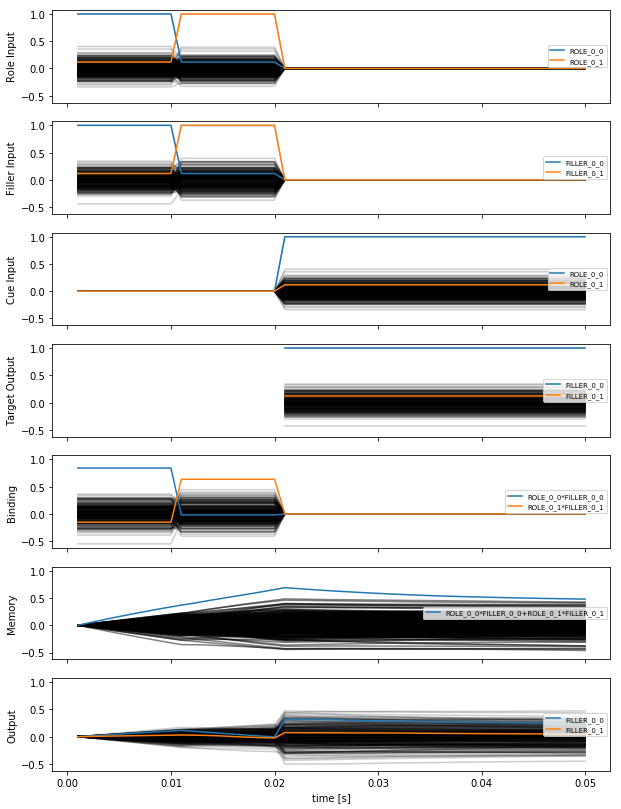
In all of these plots we are showing the similarity of the input/target/output vectors to all the items in the vocabulary, over time (highlighting the vocabulary items of interest in each case). The first three plots show the inputs to the model, and the fourth shows the desired output. The fifth and sixth plots show intermediate outputs in the model, from the first circular convolution network (which computes \(ROLE \circledast FILLER\)) and the memory (which stores a trace of all the \(ROLE \circledast FILLER\) pairs), respectively. The final plot is the actual output of the system, the \(FILLER\) corresponding to the cued \(ROLE\). Ideally this last plot should look like the “Target Output” plot, but we can see that the output accuracy is not great.
We can improve the performance of the model by optimizing its parameters using Nengo DL. As before we will download pre-trained parameters to save time, but you can run the training yourself by setting do_training=True.
[13]:
do_training = False
if do_training:
    # generate training data
    (train_roles, train_fills, train_cues, train_binding, train_memory,
     train_targets, _) = get_binding_data(8000, n_pairs, dims, seed,
                                          t_int, t_mem)

    # note: when training we'll add targets for the intermediate outputs
    # as well, to help shape the training process
    train_data = {role_inp: train_roles, fill_inp: train_fills,
                  cue_inp: train_cues,
                  output_probe: train_targets, conv_probe: train_binding,
                  memory_probe: train_memory}

    test_data = test_inputs.copy()
    test_data[output_probe] = test_targets

    # we'll define a slightly modified version of mean squared error that
    # allows us to specify a weighting (so that we can specify a
    # different weight for each probe)
    def weighted_mse(output, target, weight=1):
        target = tf.where(tf.is_nan(target), output, target)
        return weight * tf.reduce_mean(tf.square(target - output))


    with nengo_dl.Simulator(
            net, minibatch_size=minibatch_size, seed=seed) as sim:
        learning_rate = 1e-4
        optimizer = tf.train.RMSPropOptimizer(learning_rate)

        print('Test loss before:',
              sim.loss(test_data, {output_probe: nengo_dl.obj.mse}))
        sim.train(train_data, optimizer, n_epochs=10,
                  objective={output_probe: weighted_mse,
                             conv_probe: partial(weighted_mse,
                                                 weight=0.25),
                             memory_probe: partial(weighted_mse,
                                                   weight=0.25)})
        print('Test loss after:',
              sim.loss(test_data, {output_probe: nengo_dl.obj.mse}))

        sim.save_params('./mem_binding_params')
else:
    # download pretrained parameters
    urlretrieve(
        "https://drive.google.com/uc?export=download&id=1gxFE-wvEMDQZuoZq7fYM8VQEhBKHkDfD",
        "mem_binding_params.zip")
    with zipfile.ZipFile("mem_binding_params.zip") as f:
        f.extractall()
Recomputing our accuracy measure on the test inputs demonstrates that our optimization procedure has significantly improved the performance of the model.
[14]:
with nengo_dl.Simulator(
        net, seed=seed, minibatch_size=minibatch_size) as sim:
    sim.load_params('./mem_binding_params')
    sim.run(t_run, data=test_inputs)

print('Retrieval accuracy: ', accuracy(sim, output_probe, test_vocab,
                                       test_targets))
Build finished in 0:00:04
Optimization finished in 0:00:02
Construction finished in 0:00:01
Simulation finished in 0:00:00
Retrieval accuracy:  0.671875
We can visualize the change in performance by looking at the same plots as before, showing the model output for one example input trajectory.
[15]:
plot_retrieval_example(sim, test_vocab)
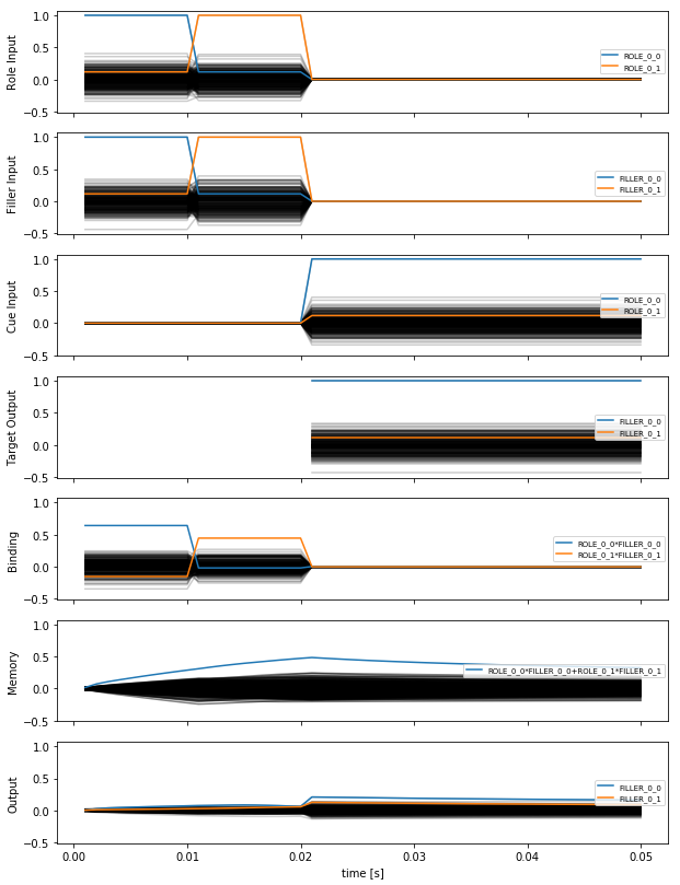
While we can see that the output of the model is not perfect, it is much closer to the target values (the most similar vocabulary item is the correct filler). You can modify various parameters of the model, such as the number of dimensions or the number of role/filler inputs, in order to see how that impacts performance.
