Communication channel

This example demonstrates how to create a connections from one neuronal ensemble to another that behaves like a communication channel (that is, it transmits information without changing it).

Network diagram:

[Input] ---> (A) ---> (B)

An abstract input signal is fed into a first neuronal ensemble \(A\), which then passes it on to another ensemble \(B\). The result is that spiking activity in ensemble \(B\) encodes the value from the Input.

import numpy as np
import matplotlib.pyplot as plt
%matplotlib inline

import nengo

Step 1: Create the Network

# Create a 'model' object to which we can add ensembles, connections, etc.
model = nengo.Network(label="Communications Channel")
with model:
    # Create an abstract input signal that oscillates as sin(t)
    sin = nengo.Node(np.sin)

    # Create the neuronal ensembles
    A = nengo.Ensemble(100, dimensions=1)
    B = nengo.Ensemble(100, dimensions=1)

    # Connect the input to the first neuronal ensemble
    nengo.Connection(sin, A)

    # Connect the first neuronal ensemble to the second
    # (this is the communication channel)
    nengo.Connection(A, B)

Step 2: Add Probes to Collect Data

Even this simple model involves many quantities that change over time, such as membrane potentials of individual neurons. Typically there are so many variables in a simulation that it is not practical to store them all. If we want to plot or analyze data from the simulation we have to “probe” the signals of interest.

with model:
    sin_probe = nengo.Probe(sin)
    A_probe = nengo.Probe(A, synapse=.01)  # ensemble output
    B_probe = nengo.Probe(B, synapse=.01)

Step 3: Run the Model!

with nengo.Simulator(model) as sim:
    sim.run(2)

Step 4: Plot the Results

plt.figure(figsize=(9, 3))
plt.subplot(1, 3, 1)
plt.title("Input")
plt.plot(sim.trange(), sim.data[sin_probe])
plt.ylim(0, 1.2)
plt.subplot(1, 3, 2)
plt.title("A")
plt.plot(sim.trange(), sim.data[A_probe])
plt.ylim(0, 1.2)
plt.subplot(1, 3, 3)
plt.title("B")
plt.plot(sim.trange(), sim.data[B_probe])
plt.ylim(0, 1.2)

(0, 1.2)

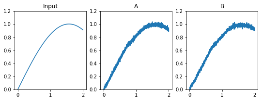
These plots show the idealized sinusoidal input, and estimates of the sinusoid that are decoded from the spiking activity of neurons in ensembles A and B.

Step 5: Using a Different Input Function

To drive the neural ensembles with different abstract inputs, it is convenient to use Python’s “Lambda Functions”. For example, try changing the sin = nengo.Node line to the following for higher-frequency input:

sin = nengo.Node(lambda t: np.sin(2*np.pi*t))