Solving the permuted sequential MNIST (psMNIST) task

The psMNIST (Permuted Sequential MNIST) task is a image classification task introduced in 2015 by Le, Jaitly, and Hinton (see paper). It is based on the Sequential MNIST task, which itself is a derivative of the MNIST task. Like the MNIST task, the goal of the psMNIST task is to have a neural network process a 28 x 28 pixel image (of a handwritten digit) into one of ten digits (0 to 9).

However, while the MNIST task presents the entire image to the network all at once, the Sequential MNIST and psMNIST tasks turn the image into a stream of 784 (28x28) individual pixels, presented to the network one at a time. The goal of the network is then to classify the pixel sequence as the appropriate digit after the last pixel has been shown. The psMNIST task adds more complexity to the input by applying a fixed permutation to all of the pixel sequences. This is done to ensure that the information contained in the image is distributed evenly throughout the sequence, so that in order to perform the task successfully, the network needs to process information across the whole length of the input sequence.

The following notebook uses a single NengoLMU layer inside a simple TensorFlow model to showcase the accuracy and efficiency of performing the psMNIST task using these novel memory cells. Using the LMU for this task currently produces state-of-the-art results this task (see paper).

%matplotlib inline

import numpy as np
import matplotlib.pyplot as plt
from IPython.display import Image, display
import tensorflow as tf

import lmu

Loading and formatting the dataset

First we set a seed to ensure that the results in this example are reproducible. A random number generator state (rng) is also created, and this will later be used to generate the fixed permutation to be applied to the image data.

seed = 0
tf.random.set_seed(seed)
np.random.seed(seed)
rng = np.random.RandomState(seed)

We now obtain the standard MNIST dataset of handwritten digits from tf.keras.datasets.

(train_images, train_labels), (
    test_images,
    test_labels,
) = tf.keras.datasets.mnist.load_data()

Downloading data from https://storage.googleapis.com/tensorflow/tf-keras-datasets/mnist.npz
11493376/11490434 [==============================] - 0s 0us/step

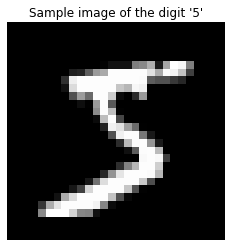
Since the pixel values of each image in the dataset have a range of 0 to 255, they are divided by 255 to change this range to 0 to 1. Let’s also display a sample image from the MNIST dataset to get an idea of the kind of images the network is working with.

train_images = train_images / 255
test_images = test_images / 255

plt.figure()
plt.imshow(np.reshape(train_images[0], (28, 28)), cmap="gray")
plt.axis("off")
plt.title(f"Sample image of the digit '{train_labels[0]}'")
plt.show()

Next, we have to convert the data from the MNIST format into the sequence of pixels that is used in the psMNIST task. To do this, we flatten the image by calling the reshape method on the images. The first dimension of the reshaped output size represents the number of samples our dataset has, which we keep the same. We want to transform each sample into a column vector, and to do so we make the second and third dimensions -1 and 1, respectively, leveraging a standard NumPy trick specifically used for converting multi-dimensional data into column vectors.

The image displayed below shows the result of this flattening process, and is an example of the type of data that is used in the Sequential MNIST task. Note that even though the image has been reshaped into an 98 x 8 image (so that it can fit on the screen), there is still a fair amount of structure observable in the image.

train_images = train_images.reshape((train_images.shape[0], -1, 1))
test_images = test_images.reshape((test_images.shape[0], -1, 1))

# we'll display the sequence in 8 rows just so that it fits better on the screen
plt.figure()
plt.imshow(train_images[0].reshape(8, -1), cmap="gray")
plt.axis("off")
plt.title(f"Sample sequence of the digit '{train_labels[0]}' (reshaped to 98 x 8)")
plt.show()

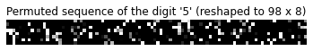
Finally, we apply a fixed permutation on the images in both the training and testing datasets. This essentially shuffles the pixels of the image sequences in a consistent way, allowing for images of the same digit to still be similar, but removing the convenience of edges and contours that the network can use for easy digit inference.

We can see, from the image below, that the fixed permutation applied to the image creates an even distribute of pixels across the entire sequence. This makes the task much more difficult as it makes it necessary for the network to process the entire input sequence to accurately predict what the digit is. We now have our data for the Permuted Sequential MNIST (psMNIST) task.

perm = rng.permutation(train_images.shape[1])
train_images = train_images[:, perm]
test_images = test_images[:, perm]

plt.figure()
plt.imshow(train_images[0].reshape(8, -1), cmap="gray")
plt.axis("off")
plt.title(f"Permuted sequence of the digit '{train_labels[0]}' (reshaped to 98 x 8)")
plt.show()

From the images in the training set, we allocate the first 50,000 images for training, and the remaining 10,000 for validation. We print out the shapes of these datasets to ensure the slicing has been done correctly.

X_train = train_images[0:50000]
X_valid = train_images[50000:]
X_test = test_images

Y_train = train_labels[0:50000]
Y_valid = train_labels[50000:]
Y_test = test_labels

print(
    f"Training inputs shape: {X_train.shape}, "
    f"Training targets shape: {Y_train.shape}"
)
print(
    f"Validation inputs shape: {X_valid.shape}, "
    f"Validation targets shape: {Y_valid.shape}"
)
print(f"Testing inputs shape: {X_test.shape}, Testing targets shape: {Y_test.shape}")

Training inputs shape: (50000, 784, 1), Training targets shape: (50000,)
Validation inputs shape: (10000, 784, 1), Validation targets shape: (10000,)
Testing inputs shape: (10000, 784, 1), Testing targets shape: (10000,)

Defining the model

Our model uses a single LMU layer configured with 212 units and an order of 256 dimensions for the memory, maintaining units + order = 468 variables in memory between time-steps. These numbers were chosen primarily to have a comparable number of internal variables to the models that were being compared against in the paper. We set theta to 784 (the number of pixels in each sequence). We also disable the hidden_to_memory and memory_to_memory connections, as based on our experimentation they are not needed/helpful in this problem.

The output of the LMU layer is connected to a Dense linear layer with an output dimensionality of 10, one for each possible digit class.

n_pixels = X_train.shape[1]

lmu_layer = tf.keras.layers.RNN(
    lmu.LMUCell(
        memory_d=1,
        order=256,
        theta=n_pixels,
        hidden_cell=tf.keras.layers.SimpleRNNCell(212),
        hidden_to_memory=False,
        memory_to_memory=False,
        input_to_hidden=True,
        kernel_initializer="ones",
    )
)

# TensorFlow layer definition
inputs = tf.keras.Input((n_pixels, 1))
lmus = lmu_layer(inputs)
outputs = tf.keras.layers.Dense(10)(lmus)

# TensorFlow model definition
model = tf.keras.Model(inputs=inputs, outputs=outputs)
model.compile(
    loss=tf.keras.losses.SparseCategoricalCrossentropy(from_logits=True),
    optimizer="adam",
    metrics=["accuracy"],
)
model.summary()

Model: "functional_1"
_________________________________________________________________
Layer (type)                 Output Shape              Param #
=================================================================
input_1 (InputLayer)         [(None, 784, 1)]          0
_________________________________________________________________
rnn (RNN)                    (None, 212)               165433
_________________________________________________________________
dense (Dense)                (None, 10)                2130
=================================================================
Total params: 167,563
Trainable params: 101,771
Non-trainable params: 65,792
_________________________________________________________________

Training the model

To train our model, we use a batch_size of 100, and train for 10 epochs, which is a far less than most other solutions to the psMNIST task. We could train for more epochs if we wished to fine-tune performance, but that is not necessary for the purposes of this example. We also create a ModelCheckpoint callback that saves the weights of the model to a file after each epoch.

The time required for this to run is tracked using the time library. Training may take a long time to complete, and to save time, this notebook defaults to using pre-trained weights. To train the model from scratch, simply change the do_training variable to True before running the cell below.

do_training = False
batch_size = 100
epochs = 10

saved_weights_fname = "./psMNIST-weights.hdf5"
callbacks = [
    tf.keras.callbacks.ModelCheckpoint(
        filepath=saved_weights_fname, monitor="val_loss", verbose=1, save_best_only=True
    ),
]

if do_training:
    result = model.fit(
        X_train,
        Y_train,
        epochs=epochs,
        batch_size=batch_size,
        validation_data=(X_valid, Y_valid),
        callbacks=callbacks,
    )

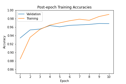
The progression of the training process is shown below. Here we plot the accuracy for the training and validation for each epoch.

Note that if this notebook has been configured to use trained weights, instead of using live data, a saved image of a previous training run will be displayed.

if do_training:
    plt.figure()
    plt.plot(result.history["val_accuracy"], label="Validation")
    plt.plot(result.history["accuracy"], label="Training")
    plt.legend()
    plt.xlabel("Epoch")
    plt.ylabel("Accuracy")
    plt.title("Post-epoch Training Accuracies")
    plt.xticks(np.arange(epochs), np.arange(1, epochs + 1))
    plt.ylim((0.85, 1.0))  # Restrict range of y axis to (0.85, 1) for readability
    plt.savefig("psMNIST-training.png")

    val_loss_min = np.argmin(result.history["val_loss"])
    print(
        f"Maximum validation accuracy: "
        f"{round(result.history['val_accuracy'][val_loss_min] * 100, 2):.2f}%"
    )

else:
    display(Image(filename="psMNIST-training.png"))

Testing the model

With the training complete, let’s use the trained weights to test the model. Since the weights are saved to file after every epoch, we can simply load the saved weights, then test it against the permuted sequences in the test set.

model.load_weights(saved_weights_fname)
accuracy = model.evaluate(X_test, Y_test)[1] * 100
print(f"Test accuracy: {round(accuracy, 2):0.2f}%")

313/313 [==============================] - 102s 327ms/step - loss: 0.1194 - accuracy: 0.9653
Test accuracy: 96.53%

As the results demonstrate, the LMU network has achieved greater than 96% accuracy on the test dataset. This is considered state-of-the-art for the psMNIST task, which is made more impressive considering the model has only been trained for 10 epochs.