
Classifying Fashion MNIST with spiking activations
![]()
This example is based on the Basic image classification example in TensorFlow. We would recommend beginning there if you would like a more basic introduction to how Keras works. In this example we will walk through how we can convert that non-spiking model into a spiking model using Keras Spiking, and various techniques that can be used to fine tune performance.
[1]:
import matplotlib.pyplot as plt
import numpy as np
import tensorflow as tf

import keras_spiking

tf.random.set_seed(0)
np.random.seed(0)
Loading data
We’ll begin by loading the Fashion MNIST data:
[2]:
(
    (train_images, train_labels),
    (test_images, test_labels),
) = tf.keras.datasets.fashion_mnist.load_data()

# normalize images so values are between 0 and 1
train_images = train_images / 255.0
test_images = test_images / 255.0

class_names = [
    "T-shirt/top",
    "Trouser",
    "Pullover",
    "Dress",
    "Coat",
    "Sandal",
    "Shirt",
    "Sneaker",
    "Bag",
    "Ankle boot",
]
num_classes = len(class_names)

plt.figure(figsize=(10, 10))
for i in range(25):
    plt.subplot(5, 5, i + 1)
    plt.imshow(train_images[i], cmap=plt.cm.binary)
    plt.axis("off")
    plt.title(class_names[train_labels[i]])

Non-spiking model
Next we’ll build and train the non-spiking model (this is identical to the original TensorFlow example).
[3]:
model = tf.keras.Sequential(
    [
        tf.keras.layers.Flatten(input_shape=(28, 28)),
        tf.keras.layers.Dense(128, activation="relu"),
        tf.keras.layers.Dense(10),
    ]
)


def train(input_model):
    input_model.compile(
        optimizer="adam",
        loss=tf.keras.losses.SparseCategoricalCrossentropy(from_logits=True),
        metrics=["accuracy"],
    )

    input_model.fit(train_images, train_labels, epochs=10)

    _, test_acc = input_model.evaluate(test_images, test_labels, verbose=2)

    print("\nTest accuracy:", test_acc)


train(model)
Epoch 1/10
1875/1875 [==============================] - 2s 1ms/step - loss: 0.4979 - accuracy: 0.8251
Epoch 2/10
1875/1875 [==============================] - 3s 1ms/step - loss: 0.3706 - accuracy: 0.8663
Epoch 3/10
1875/1875 [==============================] - 3s 2ms/step - loss: 0.3321 - accuracy: 0.8791
Epoch 4/10
1875/1875 [==============================] - 3s 2ms/step - loss: 0.3086 - accuracy: 0.8871
Epoch 5/10
1875/1875 [==============================] - 3s 2ms/step - loss: 0.2917 - accuracy: 0.8917
Epoch 6/10
1875/1875 [==============================] - 3s 2ms/step - loss: 0.2762 - accuracy: 0.8970
Epoch 7/10
1875/1875 [==============================] - 3s 2ms/step - loss: 0.2659 - accuracy: 0.9000
Epoch 8/10
1875/1875 [==============================] - 3s 2ms/step - loss: 0.2538 - accuracy: 0.9054
Epoch 9/10
1875/1875 [==============================] - 3s 2ms/step - loss: 0.2437 - accuracy: 0.9092
Epoch 10/10
1875/1875 [==============================] - 3s 2ms/step - loss: 0.2362 - accuracy: 0.9119
313/313 - 0s - loss: 0.3428 - accuracy: 0.8853

Test accuracy: 0.8852999806404114
Spiking model
Next we will create an equivalent spiking model. There are two important changes here:
Add a temporal dimension to the data/model.
Spiking models always run over time (i.e., each forward pass through the model will run for some number of timesteps). This means that we need to add a temporal dimension to the data, so instead of having shape (batch_size, ...) it will have shape (batch_size, n_steps, ...). For those familiar with working with RNNs, the principles are the same; a spiking neuron accepts temporal data and computes over time, just like an RNN.
Replace any activation functions with
keras_spiking.SpikingActivation.
keras_spiking.SpikingActivation can encapsulate any activation function, and will produce an equivalent spiking implementation. Neurons will spike at a rate proportional to the output of the base activation function. For example, if the activation function is outputting a value of 10, then the wrapped SpikingActivation will output spikes at a rate of 10Hz (i.e., 10 spikes per 1 simulated second, where 1 simulated second is equivalent to some number of timesteps, determined by the dt
parameter of SpikingActivation).
Note that for many layers, Keras combines the activation function into another layer. For example, tf.keras.layers.Dense(units=10, activation="relu") is equivalent to tf.keras.layers.Dense(units=10) -> tf.keras.layers.Activation("relu"). Due to the temporal nature of SpikingActivation it cannot be directly used within another layer as in the first case; we need to explicitly separate it into its own layer.
[4]:
# repeat the images for n_steps
n_steps = 10
train_images = np.tile(train_images[:, None], (1, n_steps, 1, 1))
test_images = np.tile(test_images[:, None], (1, n_steps, 1, 1))
[5]:
model = tf.keras.Sequential(
    [
        # add temporal dimension to the input shape; we can set it to None,
        # to allow the model to flexibly run for different lengths of time
        tf.keras.layers.Reshape((-1, 28 * 28), input_shape=(None, 28, 28)),
        # we can use Keras' TimeDistributed wrapper to allow the Dense layer
        # to operate on temporal data
        tf.keras.layers.TimeDistributed(tf.keras.layers.Dense(128)),
        # replace the "relu" activation in the non-spiking model with a
        # spiking equivalent.
        # we'll learn more about "spiking aware training" later on
        keras_spiking.SpikingActivation("relu", spiking_aware_training=False),
        # we don't need TimeDistributed on this layer, because by default
        # SpikingActivation (like all Keras RNNs) only returns the values
        # from the last timestep. we could set return_sequences=True in
        # SpikingActivation if we wanted data for all timesteps.
        tf.keras.layers.Dense(10),
    ]
)

# train the model, identically to the non-spiking version
train(model)
Epoch 1/10
1875/1875 [==============================] - 7s 4ms/step - loss: 0.5005 - accuracy: 0.8233
Epoch 2/10
1875/1875 [==============================] - 7s 4ms/step - loss: 0.3748 - accuracy: 0.8643
Epoch 3/10
1875/1875 [==============================] - 8s 4ms/step - loss: 0.3355 - accuracy: 0.8774
Epoch 4/10
1875/1875 [==============================] - 8s 4ms/step - loss: 0.3123 - accuracy: 0.8850
Epoch 5/10
1875/1875 [==============================] - 8s 4ms/step - loss: 0.2971 - accuracy: 0.8913
Epoch 6/10
1875/1875 [==============================] - 8s 4ms/step - loss: 0.2785 - accuracy: 0.8972
Epoch 7/10
1875/1875 [==============================] - 8s 4ms/step - loss: 0.2700 - accuracy: 0.8999
Epoch 8/10
1875/1875 [==============================] - 8s 4ms/step - loss: 0.2576 - accuracy: 0.9040
Epoch 9/10
1875/1875 [==============================] - 7s 4ms/step - loss: 0.2468 - accuracy: 0.9070
Epoch 10/10
1875/1875 [==============================] - 7s 4ms/step - loss: 0.2394 - accuracy: 0.9105
313/313 - 1s - loss: 16.3717 - accuracy: 0.1127

Test accuracy: 0.11270000040531158
We can see that while the training accuracy is as good as we expect, the test accuracy is not. This is due to a unique feature of SpikingActivation; it will automatically swap the behaviour of the spiking neurons during training. Because spiking neurons are (in general) not differentiable, we cannot directly use the spiking activation function during training. Instead, SpikingActivation will use the base (non-spiking) activation during training, and the spiking version during inference. So
during training above we are seeing the performance of the non-spiking model, but during evaluation we are seeing the performance of the spiking model.
So the question is, why is the performance of the spiking model so much worse than the non-spiking equivalent, and what can we do to fix that?
Simulation time
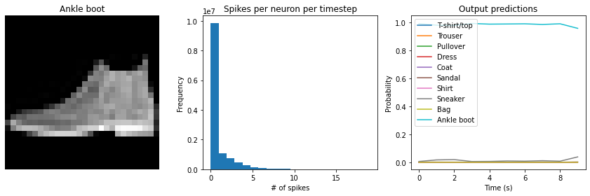
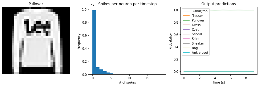
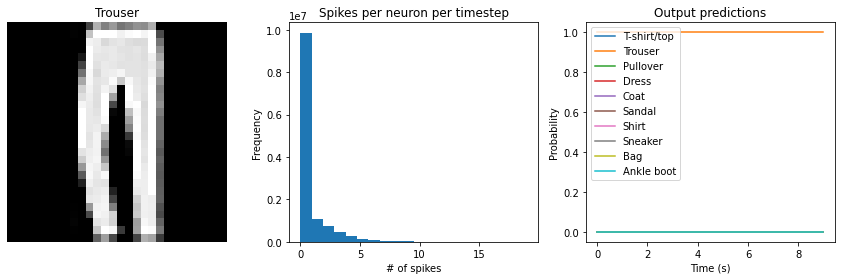
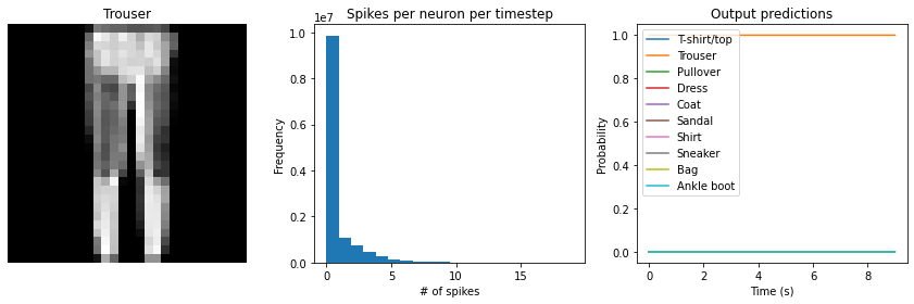
Let’s visualize the output of the spiking model, to get a better sense of what is going on.
[6]:
def check_output(seq_model, **kwargs):
"""
This code is only used for plotting purposes, and isn't necessary to
understand the rest of this example; feel free to skip it
if you just want to see the results.
"""
# rebuild the model with the functional API, so that we can
# access the output of intermediate layers
inp = x = tf.keras.Input(batch_shape=seq_model.layers[0].input_shape)
for layer in seq_model.layers:
if isinstance(layer, (keras_spiking.SpikingActivation, keras_spiking.Lowpass)):
# set return_sequences=True so we can see all the spikes,
# and update any parameters specified in kwargs
cfg = layer.get_config()
cfg["return_sequences"] = True
cfg.update(kwargs)
layer = type(layer)(**cfg)
if isinstance(layer, keras_spiking.SpikingActivation):
# save this layer so we can access it later
spike_layer = layer
x = layer(x)
func_model = tf.keras.Model(inp, [x, spike_layer.output])
# load the trained weights
func_model.set_weights(seq_model.get_weights())
# run model
output, spikes = func_model.predict(test_images)
# check test accuracy using output from last timestep
predictions = np.argmax(output[:, -1], axis=-1)
accuracy = np.equal(predictions, test_labels).mean()
print("Test accuracy: %.2f%%" % (100 * accuracy))
n_spikes = spikes * spike_layer.dt
time = spike_layer.dt * test_images.shape[1]
rates = np.sum(n_spikes, axis=1) / time
print(
"Spike rate per neuron (Hz): min=%.2f mean=%.2f max=%.2f"
% (np.min(rates), np.mean(rates), np.max(rates))
)
# plot output
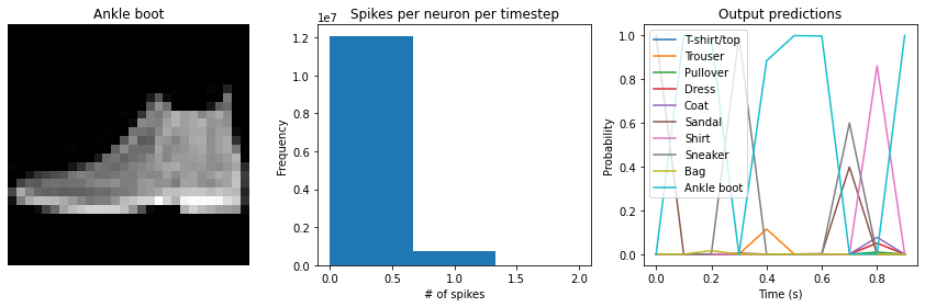
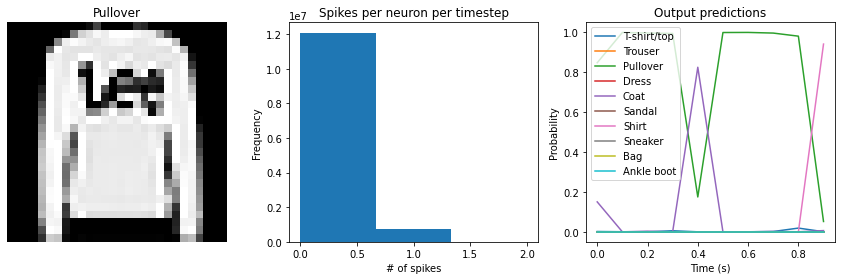
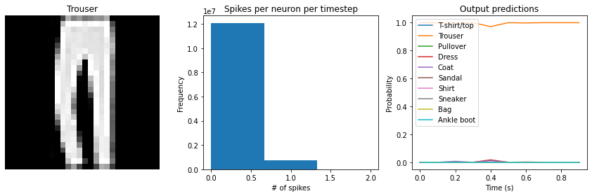
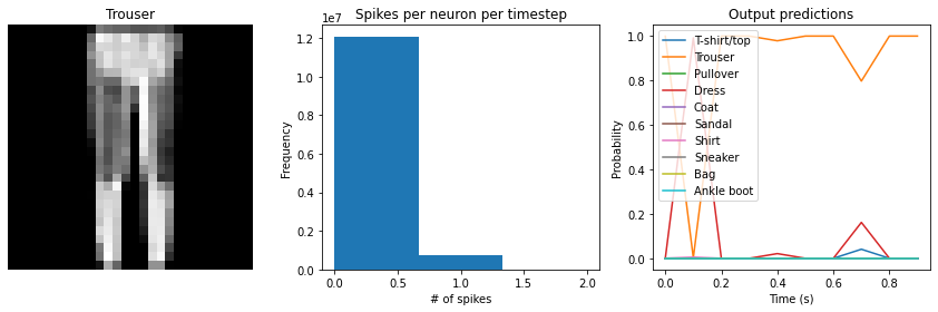
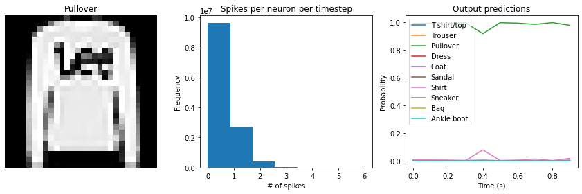
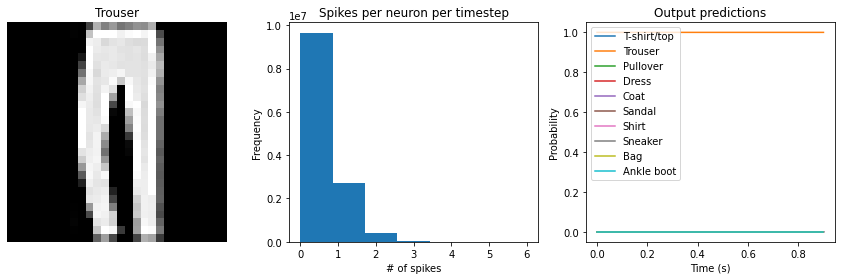
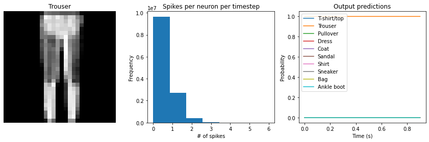
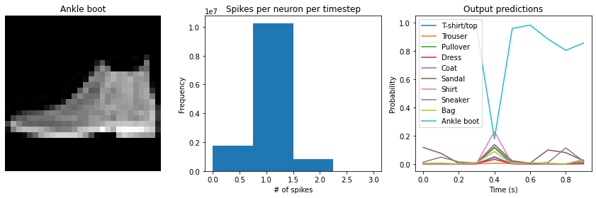
for ii in range(4):
plt.figure(figsize=(12, 4))
plt.subplot(1, 3, 1)
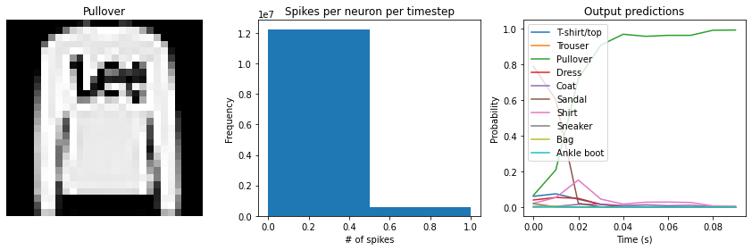
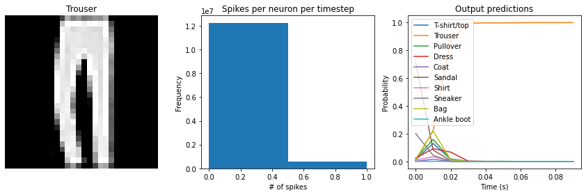
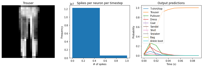
plt.title(class_names[test_labels[ii]])
plt.imshow(test_images[ii, 0], cmap="gray")
plt.axis("off")
plt.subplot(1, 3, 2)
plt.title("Spikes per neuron per timestep")
plt.hist(np.ravel(n_spikes), bins=int(np.max(n_spikes)) + 1)
plt.xlabel("# of spikes")
plt.ylabel("Frequency")
plt.subplot(1, 3, 3)
plt.title("Output predictions")
plt.plot(
np.arange(test_images.shape[1]) * spike_layer.dt, tf.nn.softmax(output[ii])
)
plt.legend(class_names, loc="upper left")
plt.xlabel("Time (s)")
plt.ylabel("Probability")
plt.ylim([-0.05, 1.05])
plt.tight_layout()
[7]:
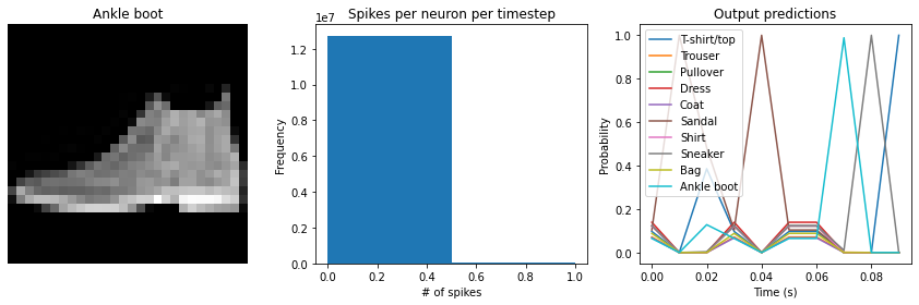
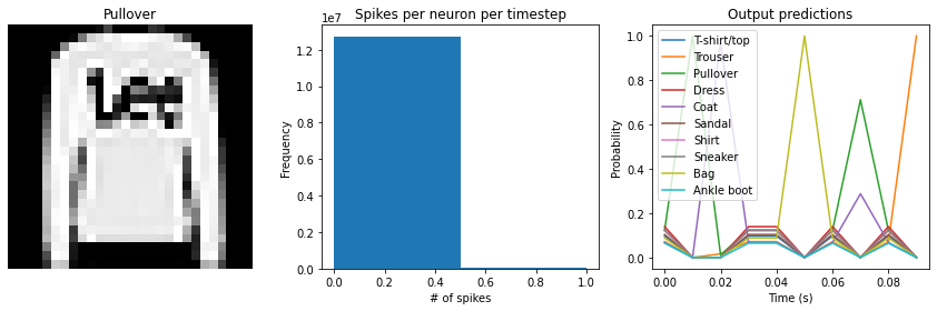
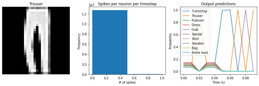
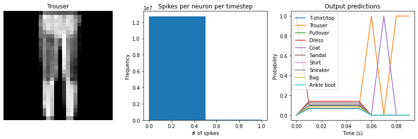
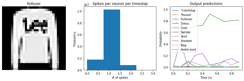
check_output(model)
Test accuracy: 11.27%
Spike rate per neuron (Hz): min=0.00 mean=0.56 max=100.00
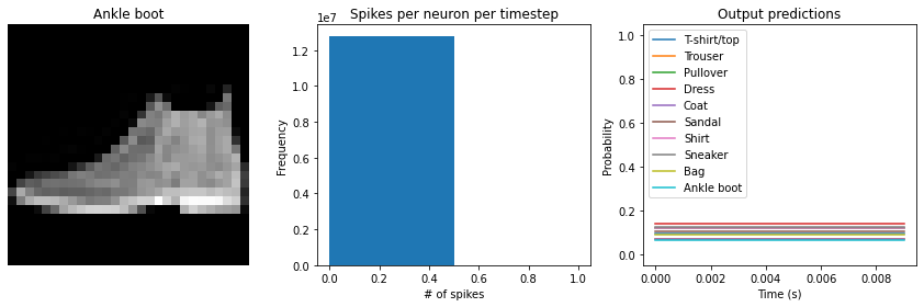
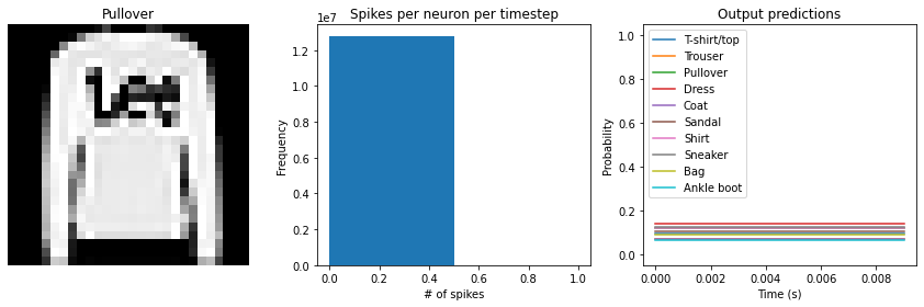
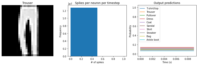
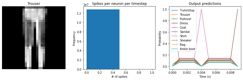
We can see an immediate problem: the neurons are hardly spiking at all. The mean number of spikes we’re getting out of each neuron in our SpikingActivation layer is much less than one, and as a result the output is mostly flat.
To help understand why, we need to think more about the temporal nature of spiking neurons. Recall that the layer is set up such that if the base activation function were to be outputting a value of 1, the spiking equivalent would be spiking at 1Hz (i.e., emitting one spike per second). In the above example we are simulating for 10 timesteps, with the default dt of 0.001s, so we’re simulating a total of 0.01s. If our neurons aren’t spiking very rapidly, and we’re only simulating for 0.01s,
then it’s not surprising that we aren’t getting any spikes in that time window.
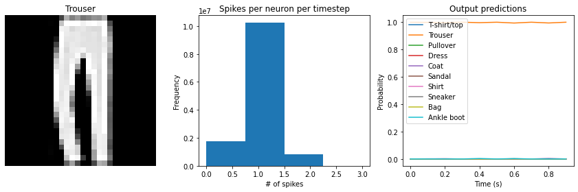
We can increase the value of dt, effectively running the spiking neurons for longer, in order to get a more accurate measure of the neuron’s output. Basically this allows us to collect more spikes from each neuron, giving us a better estimate of the neuron’s actual spike rate. We can see how the number of spikes and accuracy change as we increase dt:
[8]:
# dt=0.01 * 10 timesteps is equivalent to 0.1s of simulated time
check_output(model, dt=0.01)
Test accuracy: 19.53%
Spike rate per neuron (Hz): min=0.00 mean=0.57 max=20.00
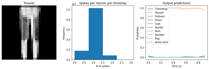
[9]:
check_output(model, dt=0.1)
Test accuracy: 65.00%
Spike rate per neuron (Hz): min=0.00 mean=0.57 max=18.00
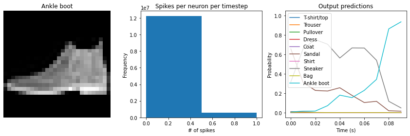
[10]:
check_output(model, dt=1)
Test accuracy: 88.21%
Spike rate per neuron (Hz): min=0.00 mean=0.57 max=18.70
We can see that as we increase dt the performance of the spiking model increasingly approaches the non-spiking performance. In addition, as dt increases, the number of spikes is increasing. To understand why this improves accuracy, keep in mind that although the simulated time is increasing, the actual number of timesteps is still 10 in all cases. We’re effectively binning all the spikes that occur on each time step. So as our bin sizes get larger (increasing dt), the spike counts
will more closely approximate the “true” output of the underlying non-spiking activation function.
One might be tempted to simply increase dt to a very large value, and thereby always get great performance. But keep in mind that when we do that we have likely lost any of the advantages that were motivating us to investigate spiking models in the first place. For example, one prominent advantage of spiking models is temporal sparsity (we only need to communicate occasional spikes, rather than continuous values). However, with large dt the neurons are likely spiking every simulation
time step (or multiple times per timestep), so the activity is no longer temporally sparse.
Thus setting dt represents a trade-off between accuracy and temporal sparsity. Choosing the appropriate value will depend on the demands of your application.
Spiking aware training
As mentioned above, by default SpikingActivation layers will use the non-spiking activation function during training and the spiking version during inference. However, similar to the idea of quantization aware training, often we can improve performance by partially incorporating spiking behaviour during training. Specifically, we will use the spiking activation on the forward pass, while still using the non-spiking version on the backwards pass. This allows the model to learn weights that account for the discrete, temporal nature of the spiking activities.
[11]:
model = tf.keras.Sequential(
    [
        tf.keras.layers.Reshape((-1, 28 * 28), input_shape=(None, 28, 28)),
        tf.keras.layers.TimeDistributed(tf.keras.layers.Dense(128)),
        # set spiking_aware training and a moderate dt
        keras_spiking.SpikingActivation("relu", dt=0.1, spiking_aware_training=True),
        tf.keras.layers.Dense(10),
    ]
)

train(model)
Epoch 1/10
1875/1875 [==============================] - 8s 4ms/step - loss: 1.0891 - accuracy: 0.6762
Epoch 2/10
1875/1875 [==============================] - 8s 4ms/step - loss: 0.6232 - accuracy: 0.7750
Epoch 3/10
1875/1875 [==============================] - 7s 3ms/step - loss: 0.5556 - accuracy: 0.8010
Epoch 4/10
1875/1875 [==============================] - 7s 3ms/step - loss: 0.5133 - accuracy: 0.8163
Epoch 5/10
1875/1875 [==============================] - 7s 4ms/step - loss: 0.4818 - accuracy: 0.8278
Epoch 6/10
1875/1875 [==============================] - 7s 4ms/step - loss: 0.4612 - accuracy: 0.8329
Epoch 7/10
1875/1875 [==============================] - 7s 4ms/step - loss: 0.4460 - accuracy: 0.8388
Epoch 8/10
1875/1875 [==============================] - 7s 4ms/step - loss: 0.4349 - accuracy: 0.8433
Epoch 9/10
1875/1875 [==============================] - 7s 4ms/step - loss: 0.4197 - accuracy: 0.8474
Epoch 10/10
1875/1875 [==============================] - 7s 4ms/step - loss: 0.4110 - accuracy: 0.8502
313/313 - 1s - loss: 0.4630 - accuracy: 0.8352

Test accuracy: 0.8352000117301941
[12]:
check_output(model)
Test accuracy: 83.52%
Spike rate per neuron (Hz): min=0.00 mean=2.86 max=56.00

We can see that with spiking_aware_training we’re getting better performance than we were with the equivalent dt value above. The model has learned weights that are less sensitive to the discrete, sparse output produced by the spiking neurons.
Spike rate regularization
As we saw in the Simulation time section, the spiking rate of the neurons is very important. If a neuron is spiking too slowly then we don’t have enough information to determine its output value. Conversely, if a neuron is spiking too quickly then we may lose the spiking advantages we are looking for, such as temporal sparsity.
Thus it can be helpful to more directly control the firing rates in the model by applying regularization penalties during training. Any of the standard Keras regularization functions can be used. Keras Spiking also includes some additional regularizers that can be useful for this case as they allow us to specify a non-zero reference point (so we can drive the activities towards some value greater than zero).
[13]:
model = tf.keras.Sequential(
    [
        tf.keras.layers.Reshape((-1, 28 * 28), input_shape=(None, 28, 28)),
        tf.keras.layers.TimeDistributed(tf.keras.layers.Dense(128)),
        keras_spiking.SpikingActivation(
            "relu",
            dt=0.1,
            spiking_aware_training=True,
            # add activity regularizer to encourage spike rates around 10Hz
            activity_regularizer=keras_spiking.L2(l2=1e-3, target=10),
        ),
        tf.keras.layers.Dense(10),
    ]
)

train(model)
Epoch 1/10
1875/1875 [==============================] - 8s 4ms/step - loss: 6.2554 - accuracy: 0.6261
Epoch 2/10
1875/1875 [==============================] - 8s 4ms/step - loss: 4.4967 - accuracy: 0.6950
Epoch 3/10
1875/1875 [==============================] - 8s 4ms/step - loss: 4.2172 - accuracy: 0.7136
Epoch 4/10
1875/1875 [==============================] - 8s 4ms/step - loss: 4.0268 - accuracy: 0.7217
Epoch 5/10
1875/1875 [==============================] - 8s 4ms/step - loss: 3.8566 - accuracy: 0.7317
Epoch 6/10
1875/1875 [==============================] - 8s 4ms/step - loss: 3.7315 - accuracy: 0.7346
Epoch 7/10
1875/1875 [==============================] - 8s 4ms/step - loss: 3.6207 - accuracy: 0.7375
Epoch 8/10
1875/1875 [==============================] - 8s 4ms/step - loss: 3.5122 - accuracy: 0.7422
Epoch 9/10
1875/1875 [==============================] - 8s 4ms/step - loss: 3.4372 - accuracy: 0.7412
Epoch 10/10
1875/1875 [==============================] - 8s 4ms/step - loss: 3.3411 - accuracy: 0.7467
313/313 - 1s - loss: 3.3676 - accuracy: 0.7252

Test accuracy: 0.7251999974250793
[14]:
check_output(model)
Test accuracy: 72.52%
Spike rate per neuron (Hz): min=0.00 mean=9.26 max=24.00
We can see that the spike rates have moved towards the 10Hz target we specified. However, the test accuracy has dropped, since we’re adding an additional optimization constraint. Again this is a tradeoff that is made between controlling the firing rates and optimizing accuracy, and the best value for that tradeoff will depend on the particular application (e.g., how important is it that spike rates fall within a particular range?).
Lowpass filtering
Another tool we can employ when working with SpikingActivation layers is filtering. As we’ve seen, the output of a spiking layer consists of discrete, temporally sparse spike events. This makes it difficult to determine the spike rate of a neuron when just looking at a single timestep. For example, in the cases above we are only using the output on the final timestep to compute the test accuracy. But it’s possible that a neuron that actually has a low spike rate just happened to spike on that final timestep, throwing off our measured results.
It seems natural then, rather than just looking at a single timestep, to compute some kind of moving average of the spiking output across timesteps. This is effectively what filtering is doing. Keras Spiking contains a Lowpass layer, which implements a lowpass filter. This has a parameter tau, known as the filter time constant, which controls the degree of smoothing the layer will apply. Larger tau values will apply more smoothing,
meaning that we’re aggregating information across longer periods of time, but the output will also be slower to adapt to changes in the input.
By default the tau values are trainable. We can use this in combination with spiking aware training to enable the model to learn time constants that best trade off spike noise versus response speed.
[15]:
model = tf.keras.Sequential(
    [
        tf.keras.layers.Reshape((-1, 28 * 28), input_shape=(None, 28, 28)),
        tf.keras.layers.TimeDistributed(tf.keras.layers.Dense(128)),
        # we'll use a smaller dt value of 0.01
        # note: we set return_sequences=True, because we want to pass the whole sequence
        # of spikes to Lowpass to be filtered
        keras_spiking.SpikingActivation(
            "relu", return_sequences=True, spiking_aware_training=True, dt=0.01
        ),
        # add a lowpass filter on output of spiking layer
        # note: the lowpass dt doesn't necessarily need to be the same as the
        # SpikingActivation dt, but it's probably a good idea to keep them in sync
        # so that if we change dt the relative effect of the lowpass filter is unchanged
        keras_spiking.Lowpass(tau=0.1, dt=0.01),
        tf.keras.layers.Dense(10),
    ]
)

train(model)
Epoch 1/10
1875/1875 [==============================] - 14s 8ms/step - loss: 0.9261 - accuracy: 0.6963
Epoch 2/10
1875/1875 [==============================] - 15s 8ms/step - loss: 0.5883 - accuracy: 0.7857
Epoch 3/10
1875/1875 [==============================] - 15s 8ms/step - loss: 0.5242 - accuracy: 0.8110
Epoch 4/10
1875/1875 [==============================] - 15s 8ms/step - loss: 0.4822 - accuracy: 0.8265
Epoch 5/10
1875/1875 [==============================] - 16s 9ms/step - loss: 0.4563 - accuracy: 0.8352
Epoch 6/10
1875/1875 [==============================] - 16s 8ms/step - loss: 0.4386 - accuracy: 0.8417
Epoch 7/10
1875/1875 [==============================] - 16s 9ms/step - loss: 0.4227 - accuracy: 0.8467
Epoch 8/10
1875/1875 [==============================] - 16s 9ms/step - loss: 0.4107 - accuracy: 0.8494
Epoch 9/10
1875/1875 [==============================] - 16s 9ms/step - loss: 0.3946 - accuracy: 0.8564
Epoch 10/10
1875/1875 [==============================] - 16s 9ms/step - loss: 0.3868 - accuracy: 0.8582
313/313 - 1s - loss: 0.4297 - accuracy: 0.8501

Test accuracy: 0.8500999808311462
[16]:
check_output(model)
Test accuracy: 85.01%
Spike rate per neuron (Hz): min=0.00 mean=4.30 max=70.00
We can see that we are getting roughly equivalent performance to the previous spiking aware training example, but with much fewer spikes (because we’re using 1/10th the dt). That is, we can be more aggressive in our temporal sparsification, because we’re using the Lowpass filtering to aggregate information over time.
Summary
We can use SpikingActivation layers to convert any activation function to an equivalent spiking implementation. Models with SpikingActivations can be trained and evaluated in the same way as non-spiking models, thanks to the swappable training/inference behaviour.
There are also a number of additional features that should be kept in mind in order to optimize the performance of a spiking model:
Simulation time: by adjusting
dtwe can trade off temporal sparsity versus accuracySpiking aware training: incorporating spiking dynamics on the forward pass can allow the model to learn weights that are more robust to spiking activations
Spike rate regularization: we can gain more control over spike rates by directly incorporating activity regularization into the optimization process
Lowpass filtering: we can achieve better accuracy with fewer spikes by aggregating spike data over time