Classifying Fashion MNIST with spiking activations
![]()
This example is based on the Basic image classification example in TensorFlow. We would recommend beginning there if you would like a more basic introduction to how Keras works. In this example we will walk through how we can convert that non-spiking model into a spiking model using KerasSpiking, and various techniques that can be used to fine tune performance.
[1]:
import matplotlib.pyplot as plt
import numpy as np
import tensorflow as tf

import keras_spiking

tf.random.set_seed(0)
np.random.seed(0)
Loading data
We’ll begin by loading the Fashion MNIST data:
[2]:
(
    (train_images, train_labels),
    (test_images, test_labels),
) = tf.keras.datasets.fashion_mnist.load_data()

# normalize images so values are between 0 and 1
train_images = train_images / 255.0
test_images = test_images / 255.0

class_names = [
    "T-shirt/top",
    "Trouser",
    "Pullover",
    "Dress",
    "Coat",
    "Sandal",
    "Shirt",
    "Sneaker",
    "Bag",
    "Ankle boot",
]
num_classes = len(class_names)

plt.figure(figsize=(10, 10))
for i in range(25):
    plt.subplot(5, 5, i + 1)
    plt.imshow(train_images[i], cmap=plt.cm.binary)
    plt.axis("off")
    plt.title(class_names[train_labels[i]])

Non-spiking model
Next we’ll build and train the non-spiking model (this is identical to the original TensorFlow example).
[3]:
model = tf.keras.Sequential(
    [
        tf.keras.layers.Flatten(input_shape=(28, 28)),
        tf.keras.layers.Dense(128, activation="relu"),
        tf.keras.layers.Dense(10),
    ]
)


def train(input_model, train_x, test_x):
    input_model.compile(
        optimizer="adam",
        loss=tf.keras.losses.SparseCategoricalCrossentropy(from_logits=True),
        metrics=["accuracy"],
    )

    input_model.fit(train_x, train_labels, epochs=10)

    _, test_acc = input_model.evaluate(test_x, test_labels, verbose=2)

    print("\nTest accuracy:", test_acc)


train(model, train_images, test_images)
2021-11-09 00:43:09.254608: I tensorflow/core/platform/cpu_feature_guard.cc:151] This TensorFlow binary is optimized with oneAPI Deep Neural Network Library (oneDNN) to use the following CPU instructions in performance-critical operations:  AVX2 FMA
To enable them in other operations, rebuild TensorFlow with the appropriate compiler flags.
2021-11-09 00:43:09.820968: I tensorflow/core/common_runtime/gpu/gpu_device.cc:1525] Created device /job:localhost/replica:0/task:0/device:GPU:0 with 10792 MB memory:  -> device: 0, name: Tesla K80, pci bus id: 0001:00:00.0, compute capability: 3.7
Epoch 1/10
1875/1875 [==============================] - 4s 2ms/step - loss: 0.4979 - accuracy: 0.8250
Epoch 2/10
1875/1875 [==============================] - 3s 2ms/step - loss: 0.3703 - accuracy: 0.8653
Epoch 3/10
1875/1875 [==============================] - 3s 2ms/step - loss: 0.3318 - accuracy: 0.8795
Epoch 4/10
1875/1875 [==============================] - 3s 2ms/step - loss: 0.3082 - accuracy: 0.8868
Epoch 5/10
1875/1875 [==============================] - 3s 2ms/step - loss: 0.2920 - accuracy: 0.8918
Epoch 6/10
1875/1875 [==============================] - 3s 2ms/step - loss: 0.2763 - accuracy: 0.8979
Epoch 7/10
1875/1875 [==============================] - 3s 2ms/step - loss: 0.2666 - accuracy: 0.9001
Epoch 8/10
1875/1875 [==============================] - 3s 2ms/step - loss: 0.2545 - accuracy: 0.9065
Epoch 9/10
1875/1875 [==============================] - 3s 2ms/step - loss: 0.2450 - accuracy: 0.9084
Epoch 10/10
1875/1875 [==============================] - 3s 2ms/step - loss: 0.2367 - accuracy: 0.9115
313/313 - 1s - loss: 0.3424 - accuracy: 0.8832 - 538ms/epoch - 2ms/step

Test accuracy: 0.8831999897956848
Spiking model
Next we will create an equivalent spiking model. There are three important changes here:
Add a temporal dimension to the data/model.
Spiking models always run over time (i.e., each forward pass through the model will run for some number of timesteps). This means that we need to add a temporal dimension to the data, so instead of having shape (batch_size, ...) it will have shape (batch_size, n_steps, ...). For those familiar with working with RNNs, the principles are the same; a spiking neuron accepts temporal data and computes over time, just like an RNN.
Replace any activation functions with
keras_spiking.SpikingActivation.
keras_spiking.SpikingActivation can encapsulate any activation function, and will produce an equivalent spiking implementation. Neurons will spike at a rate proportional to the output of the base activation function. For example, if the activation function is outputting a value of 10, then the wrapped SpikingActivation will output spikes at a rate of 10Hz (i.e., 10 spikes per 1 simulated second, where 1 simulated second is equivalent to some number of timesteps, determined by the dt
parameter of SpikingActivation).
Note that for many layers, Keras combines the activation function into another layer. For example, tf.keras.layers.Dense(units=10, activation="relu") is equivalent to tf.keras.layers.Dense(units=10) -> tf.keras.layers.Activation("relu"). Due to the temporal nature of SpikingActivation it cannot be directly used within another layer as in the first case; we need to explicitly separate it into its own layer.
Pool across time
The output of our keras_spiking.SpikingActivation layer is also a timeseries. For classification, we need to aggregate that temporal information somehow to generate a final prediction. Averaging the output over time is usually a good approach (but not the only method; we could also, e.g., look at the output on the last timestep or the time to first spike). We add a tf.keras.layers.GlobalAveragePooling1D layer to average across the temporal dimension of the data.
[4]:
# repeat the images for n_steps
n_steps = 10
train_sequences = np.tile(train_images[:, None], (1, n_steps, 1, 1))
test_sequences = np.tile(test_images[:, None], (1, n_steps, 1, 1))
[5]:
spiking_model = tf.keras.Sequential(
    [
        # add temporal dimension to the input shape; we can set it to None,
        # to allow the model to flexibly run for different lengths of time
        tf.keras.layers.Reshape((-1, 28 * 28), input_shape=(None, 28, 28)),
        # we can use Keras' TimeDistributed wrapper to allow the Dense layer
        # to operate on temporal data
        tf.keras.layers.TimeDistributed(tf.keras.layers.Dense(128)),
        # replace the "relu" activation in the non-spiking model with a
        # spiking equivalent
        keras_spiking.SpikingActivation("relu", spiking_aware_training=False),
        # use average pooling layer to average spiking output over time
        tf.keras.layers.GlobalAveragePooling1D(),
        tf.keras.layers.Dense(10),
    ]
)

# train the model, identically to the non-spiking version,
# except using the time sequences as inputs
train(spiking_model, train_sequences, test_sequences)
Epoch 1/10
1875/1875 [==============================] - 9s 4ms/step - loss: 0.5006 - accuracy: 0.8229
Epoch 2/10
1875/1875 [==============================] - 8s 4ms/step - loss: 0.3738 - accuracy: 0.8643
Epoch 3/10
1875/1875 [==============================] - 8s 4ms/step - loss: 0.3357 - accuracy: 0.8772
Epoch 4/10
1875/1875 [==============================] - 8s 4ms/step - loss: 0.3115 - accuracy: 0.8845
Epoch 5/10
1875/1875 [==============================] - 8s 4ms/step - loss: 0.2962 - accuracy: 0.8907
Epoch 6/10
1875/1875 [==============================] - 8s 4ms/step - loss: 0.2796 - accuracy: 0.8968
Epoch 7/10
1875/1875 [==============================] - 8s 4ms/step - loss: 0.2701 - accuracy: 0.9002
Epoch 8/10
1875/1875 [==============================] - 8s 4ms/step - loss: 0.2586 - accuracy: 0.9041
Epoch 9/10
1875/1875 [==============================] - 8s 4ms/step - loss: 0.2467 - accuracy: 0.9078
Epoch 10/10
1875/1875 [==============================] - 8s 4ms/step - loss: 0.2403 - accuracy: 0.9100
313/313 - 1s - loss: 10.8111 - accuracy: 0.1955 - 953ms/epoch - 3ms/step

Test accuracy: 0.19550000131130219
We can see that while the training accuracy is as good as we expect, the test accuracy is not. This is due to a unique feature of SpikingActivation; it will automatically swap the behaviour of the spiking neurons during training. Because spiking neurons are (in general) not differentiable, we cannot directly use the spiking activation function during training. Instead, SpikingActivation will use the base (non-spiking) activation during training, and the spiking version during inference. So
during training above we are seeing the performance of the non-spiking model, but during evaluation we are seeing the performance of the spiking model.
So the question is, why is the performance of the spiking model so much worse than the non-spiking equivalent, and what can we do to fix that?
Simulation time
Let’s visualize the output of the spiking model, to get a better sense of what is going on.
[6]:
def check_output(seq_model, modify_dt=None):
"""
This code is only used for plotting purposes, and isn't necessary to
understand the rest of this example; feel free to skip it
if you just want to see the results.
"""
# rebuild the model with the functional API, so that we can
# access the output of intermediate layers
inp = x = tf.keras.Input(batch_shape=seq_model.layers[0].input_shape)
has_global_average_pooling = False
for layer in seq_model.layers:
if isinstance(layer, tf.keras.layers.GlobalAveragePooling1D):
# remove the pooling so that we can see the model's
# output over time
has_global_average_pooling = True
continue
if isinstance(layer, (keras_spiking.SpikingActivation, keras_spiking.Lowpass)):
cfg = layer.get_config()
# update dt, if specified
if modify_dt is not None:
cfg["dt"] = modify_dt
# always return the full time series so we can visualize it
cfg["return_sequences"] = True
layer = type(layer)(**cfg)
if isinstance(layer, keras_spiking.SpikingActivation):
# save this layer so we can access it later
spike_layer = layer
x = layer(x)
func_model = tf.keras.Model(inp, [x, spike_layer.output])
# copy weights to new model
func_model.set_weights(seq_model.get_weights())
# run model
output, spikes = func_model.predict(test_sequences)
if has_global_average_pooling:
# check test accuracy using average output over all timesteps
predictions = np.argmax(output.mean(axis=1), axis=-1)
else:
# check test accuracy using output from only the last timestep
predictions = np.argmax(output[:, -1], axis=-1)
accuracy = np.equal(predictions, test_labels).mean()
print(f"Test accuracy: {100 * accuracy:.2f}%")
time = test_sequences.shape[1] * spike_layer.dt
n_spikes = spikes * spike_layer.dt
rates = np.sum(n_spikes, axis=1) / time
print(
f"Spike rate per neuron (Hz): min={np.min(rates):.2f} "
f"mean={np.mean(rates):.2f} max={np.max(rates):.2f}"
)
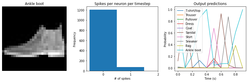
# plot output
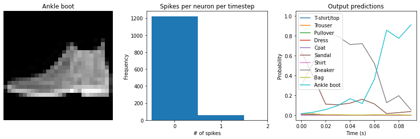
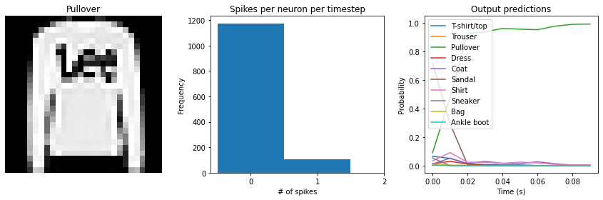
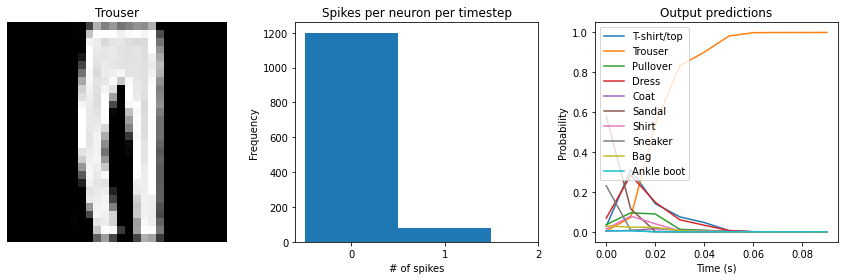
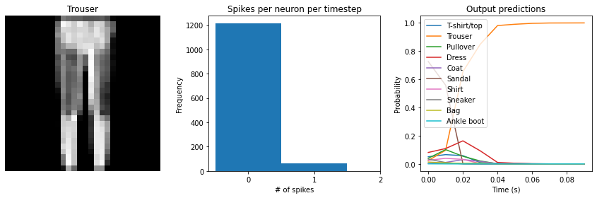
for ii in range(4):
plt.figure(figsize=(12, 4))
plt.subplot(1, 3, 1)
plt.title(class_names[test_labels[ii]])
plt.imshow(test_images[ii], cmap="gray")
plt.axis("off")
plt.subplot(1, 3, 2)
plt.title("Spikes per neuron per timestep")
bin_edges = np.arange(int(np.max(n_spikes[ii])) + 2) - 0.5
plt.hist(np.ravel(n_spikes[ii]), bins=bin_edges)
x_ticks = plt.xticks()[0]
plt.xticks(
x_ticks[(np.abs(x_ticks - np.round(x_ticks)) < 1e-8) & (x_ticks > -1e-8)]
)
plt.xlabel("# of spikes")
plt.ylabel("Frequency")
plt.subplot(1, 3, 3)
plt.title("Output predictions")
plt.plot(
np.arange(test_sequences.shape[1]) * spike_layer.dt,
tf.nn.softmax(output[ii]),
)
plt.legend(class_names, loc="upper left")
plt.xlabel("Time (s)")
plt.ylabel("Probability")
plt.ylim([-0.05, 1.05])
plt.tight_layout()
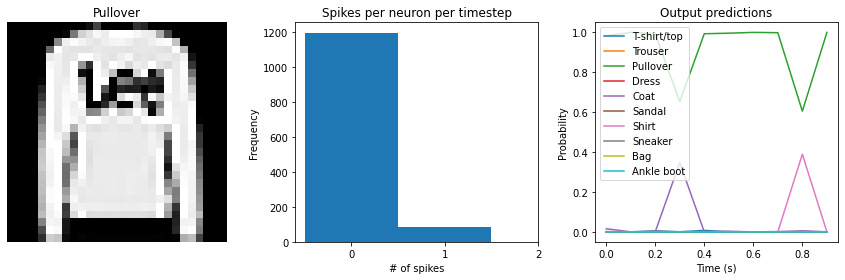
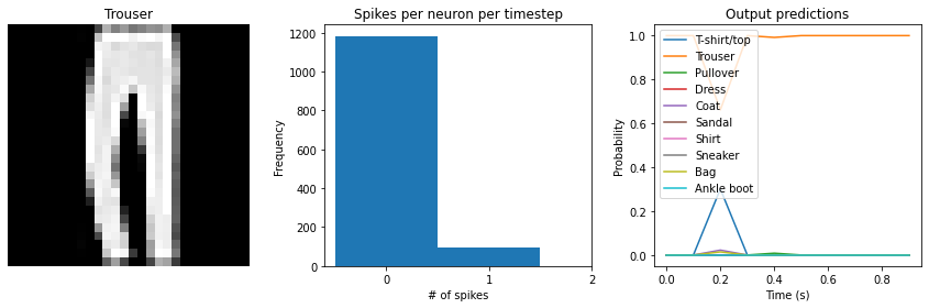
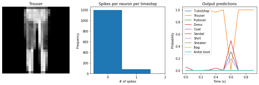
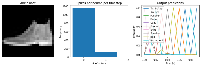
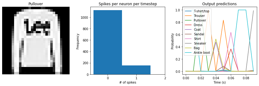
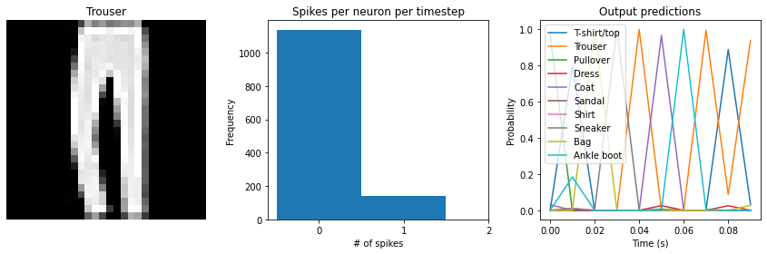
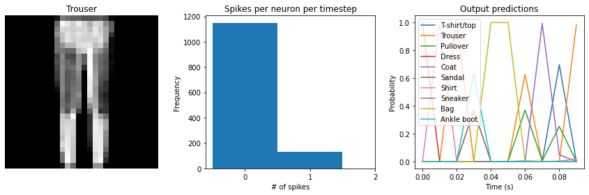
[7]:
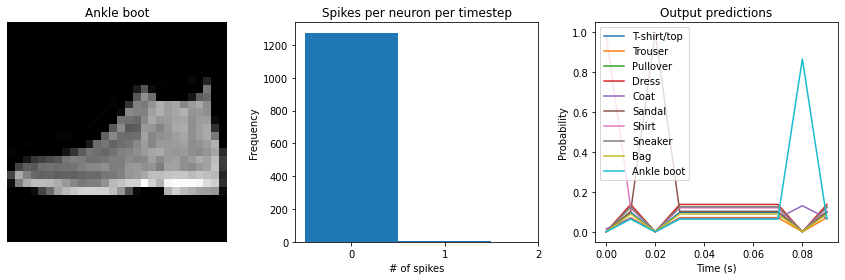
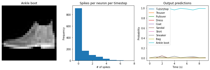
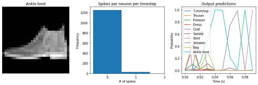
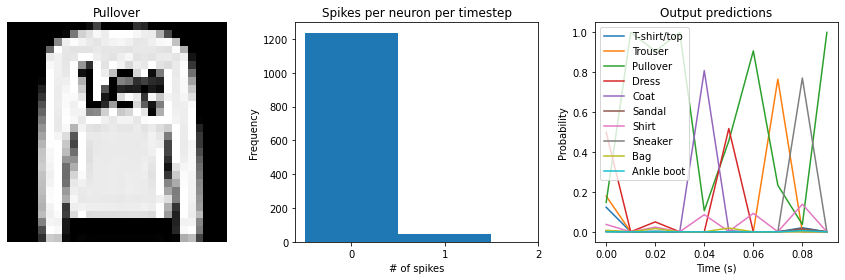
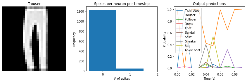
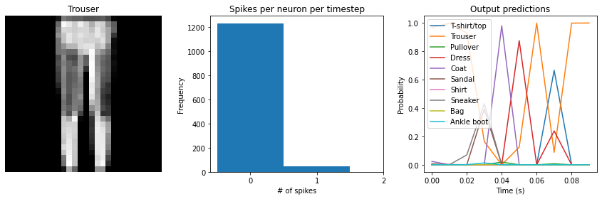
check_output(spiking_model)
Test accuracy: 19.55%
Spike rate per neuron (Hz): min=0.00 mean=0.52 max=100.00
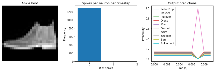
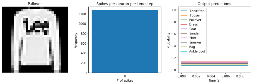
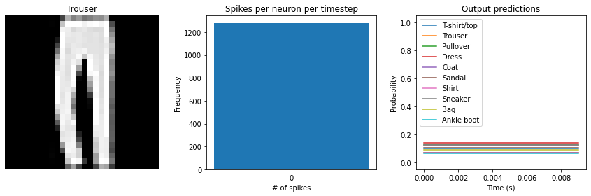
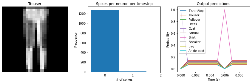
We can see an immediate problem: the neurons are hardly spiking at all. The mean number of spikes we’re getting out of each neuron in our SpikingActivation layer is much less than one, and as a result the output is mostly flat.
To help understand why, we need to think more about the temporal nature of spiking neurons. Recall that the layer is set up such that if the base activation function were to be outputting a value of 1, the spiking equivalent would be spiking at 1Hz (i.e., emitting one spike per second). In the above example we are simulating for 10 timesteps, with the default dt of 0.001s, so we’re simulating a total of 0.01s. If our neurons aren’t spiking very rapidly, and we’re only simulating for 0.01s,
then it’s not surprising that we aren’t getting any spikes in that time window.
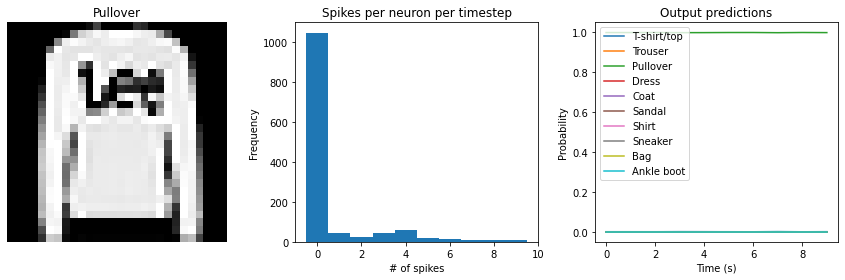
We can increase the value of dt, effectively running the spiking neurons for longer, in order to get a more accurate measure of the neuron’s output. Basically this allows us to collect more spikes from each neuron, giving us a better estimate of the neuron’s actual spike rate. We can see how the number of spikes and accuracy change as we increase dt:
[8]:
# dt=0.01 * 10 timesteps is equivalent to 0.1s of simulated time
check_output(spiking_model, modify_dt=0.01)
Test accuracy: 64.43%
Spike rate per neuron (Hz): min=0.00 mean=0.53 max=20.00
[9]:
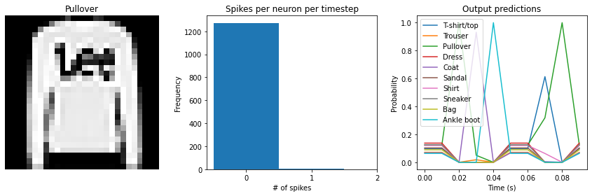
check_output(spiking_model, modify_dt=0.1)
Test accuracy: 88.14%
Spike rate per neuron (Hz): min=0.00 mean=0.53 max=15.00
[10]:
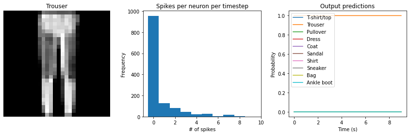
check_output(spiking_model, modify_dt=1)
Test accuracy: 88.37%
Spike rate per neuron (Hz): min=0.00 mean=0.53 max=14.40
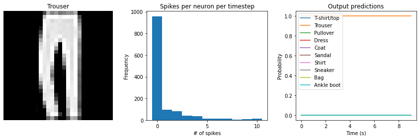
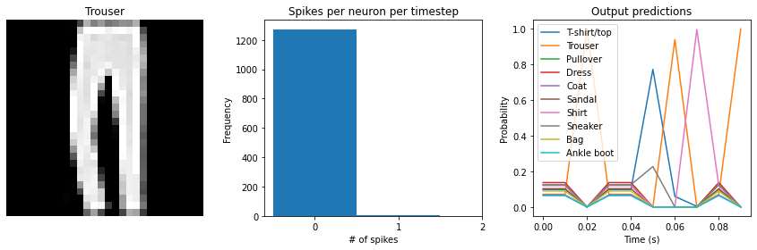
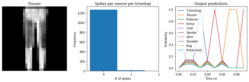
We can see that as we increase dt the performance of the spiking model increasingly approaches the non-spiking performance. In addition, as dt increases, the number of spikes is increasing. To understand why this improves accuracy, keep in mind that although the simulated time is increasing, the actual number of timesteps is still 10 in all cases. We’re effectively binning all the spikes that occur on each time step. So as our bin sizes get larger (increasing dt), the spike counts
will more closely approximate the “true” output of the underlying non-spiking activation function.
One might be tempted to simply increase dt to a very large value, and thereby always get great performance. But keep in mind that when we do that we have likely lost any of the advantages that were motivating us to investigate spiking models in the first place. For example, one prominent advantage of spiking models is temporal sparsity (we only need to communicate occasional spikes, rather than continuous values). However, with large dt the neurons are likely spiking every simulation
time step (or multiple times per timestep), so the activity is no longer temporally sparse.
Thus setting dt represents a trade-off between accuracy and temporal sparsity. Choosing the appropriate value will depend on the demands of your application.
In some cases it can be useful to modify dt over the course of training. For example, we could start with a large dt and then gradually decrease it over time. See keras_spiking.callbacks.DtScheduler for more details.
Spiking aware training
As mentioned above, by default SpikingActivation layers will use the non-spiking activation function during training and the spiking version during inference. However, similar to the idea of quantization aware training, often we can improve performance by partially incorporating spiking behaviour during training. Specifically, we will use the spiking activation on the forward pass, while still using the non-spiking version on the backwards pass. This allows the model to learn weights that account for the discrete, temporal nature of the spiking activities.
[11]:
spikeaware_model = tf.keras.Sequential(
    [
        tf.keras.layers.Reshape((-1, 28 * 28), input_shape=(None, 28, 28)),
        tf.keras.layers.TimeDistributed(tf.keras.layers.Dense(128)),
        # set spiking_aware training and a moderate dt
        keras_spiking.SpikingActivation("relu", dt=0.01, spiking_aware_training=True),
        tf.keras.layers.GlobalAveragePooling1D(),
        tf.keras.layers.Dense(10),
    ]
)

train(spikeaware_model, train_sequences, test_sequences)
Epoch 1/10
1875/1875 [==============================] - 10s 5ms/step - loss: 1.0956 - accuracy: 0.6776
Epoch 2/10
1875/1875 [==============================] - 9s 5ms/step - loss: 0.6272 - accuracy: 0.7746
Epoch 3/10
1875/1875 [==============================] - 9s 5ms/step - loss: 0.5530 - accuracy: 0.8013
Epoch 4/10
1875/1875 [==============================] - 9s 5ms/step - loss: 0.5085 - accuracy: 0.8180
Epoch 5/10
1875/1875 [==============================] - 9s 5ms/step - loss: 0.4812 - accuracy: 0.8257
Epoch 6/10
1875/1875 [==============================] - 9s 5ms/step - loss: 0.4604 - accuracy: 0.8340
Epoch 7/10
1875/1875 [==============================] - 8s 4ms/step - loss: 0.4460 - accuracy: 0.8401
Epoch 8/10
1875/1875 [==============================] - 9s 5ms/step - loss: 0.4321 - accuracy: 0.8454
Epoch 9/10
1875/1875 [==============================] - 8s 5ms/step - loss: 0.4189 - accuracy: 0.8471
Epoch 10/10
1875/1875 [==============================] - 8s 4ms/step - loss: 0.4094 - accuracy: 0.8515
313/313 - 1s - loss: 0.4484 - accuracy: 0.8427 - 967ms/epoch - 3ms/step

Test accuracy: 0.8427000045776367
[12]:
check_output(spikeaware_model)
Test accuracy: 84.27%
Spike rate per neuron (Hz): min=0.00 mean=2.74 max=50.00
We can see that with spiking_aware_training we’re getting better performance than we were with the equivalent dt value above. The model has learned weights that are less sensitive to the discrete, sparse output produced by the spiking neurons.
Spike rate regularization
As we saw in the Simulation time section, the spiking rate of the neurons is very important. If a neuron is spiking too slowly then we don’t have enough information to determine its output value. Conversely, if a neuron is spiking too quickly then we may lose the spiking advantages we are looking for, such as temporal sparsity.
Thus it can be helpful to more directly control the firing rates in the model by applying regularization penalties during training. Any of the standard Keras regularization functions can be used. KerasSpiking also includes some additional regularizers that can be useful for this case as they allow us to specify a non-zero reference point (so we can drive the activities towards some value greater than zero), or a range of acceptable values.
[13]:
regularized_model = tf.keras.Sequential(
    [
        tf.keras.layers.Reshape((-1, 28 * 28), input_shape=(None, 28, 28)),
        tf.keras.layers.TimeDistributed(tf.keras.layers.Dense(128)),
        keras_spiking.SpikingActivation(
            "relu",
            dt=0.01,
            spiking_aware_training=True,
            # add activity regularizer to encourage spike rates between 10 and 20 Hz
            activity_regularizer=keras_spiking.regularizers.L2(
                l2=1e-4, target=(10, 20)
            ),
        ),
        tf.keras.layers.GlobalAveragePooling1D(),
        tf.keras.layers.Dense(10),
    ]
)

train(regularized_model, train_sequences, test_sequences)
Epoch 1/10
1875/1875 [==============================] - 9s 5ms/step - loss: 83.6276 - accuracy: 0.6255
Epoch 2/10
1875/1875 [==============================] - 9s 5ms/step - loss: 89.5422 - accuracy: 0.6953
Epoch 3/10
1875/1875 [==============================] - 9s 5ms/step - loss: 90.6554 - accuracy: 0.7155
Epoch 4/10
1875/1875 [==============================] - 9s 5ms/step - loss: 91.3400 - accuracy: 0.7250
Epoch 5/10
1875/1875 [==============================] - 9s 5ms/step - loss: 91.8324 - accuracy: 0.7311
Epoch 6/10
1875/1875 [==============================] - 9s 5ms/step - loss: 92.2763 - accuracy: 0.7427
Epoch 7/10
1875/1875 [==============================] - 9s 5ms/step - loss: 92.6100 - accuracy: 0.7442
Epoch 8/10
1875/1875 [==============================] - 9s 5ms/step - loss: 92.9052 - accuracy: 0.7455
Epoch 9/10
1875/1875 [==============================] - 9s 5ms/step - loss: 93.1737 - accuracy: 0.7467
Epoch 10/10
1875/1875 [==============================] - 9s 5ms/step - loss: 93.4364 - accuracy: 0.7498
313/313 - 1s - loss: 93.4132 - accuracy: 0.7519 - 997ms/epoch - 3ms/step

Test accuracy: 0.7519000172615051
[14]:
check_output(regularized_model)
Test accuracy: 75.19%
Spike rate per neuron (Hz): min=0.00 mean=9.91 max=30.00
We can see that the spike rates have moved towards the 10-20 Hz target we specified. However, the test accuracy has dropped, since we’re adding an additional optimization constraint. (The accuracy is still higher than the original result with dt=0.01, due to the higher spike rates.) We could lower the regularization weight to allow more freedom in the firing rates. Or we could use keras_spiking.regularizers.Percentile, which allows more freedom for outliers. Again, this is a tradeoff
that is made between controlling the firing rates and optimizing accuracy, and the best value for that tradeoff will depend on the particular application (e.g., how important is it that spike rates fall within a particular range?).
Note that in some cases it may be better to use regularization with spiking_aware_training=False, as the regularization may perform better when the value being regularized is smoother. It may also help to adjust the weight initialization so that the initial firing rates are closer to the desired range, so that there are smaller adjustments required by the regularizer.
Lowpass filtering
Another tool we can employ when working with SpikingActivation layers is filtering. As we’ve seen, the output of a spiking layer consists of discrete, temporally sparse spike events. This makes it difficult to determine the spike rate of a neuron when just looking at a single timestep. In the cases above we have worked around this by using a tf.keras.layers.GlobalAveragePooling1D layer to average the output across all timesteps before classification.
Another way to achieve this is to compute some kind of moving average of the spiking output across timesteps. This is effectively what filtering is doing. KerasSpiking contains a Lowpass layer, which implements a lowpass filter. This has a parameter tau, known as the filter time constant, which controls the degree of smoothing the layer will apply. Larger tau values will apply more smoothing, meaning that we’re aggregating information
across longer periods of time, but the output will also be slower to adapt to changes in the input.
By default the tau values are trainable. We can use this in combination with spiking aware training to enable the model to learn time constants that best trade off spike noise versus response speed.
Unlike tf.keras.layers.GlobalAveragePooling1D, keras_spiking.Lowpass computes outputs for all timesteps by default. This makes it possible to apply filtering throughout the model—not only on the final layer—in the case that there are multiple spiking layers. For the final layer, we can pass return_sequences=False to have the layer only return the output of the final timestep, rather than the outputs of all timesteps.
When working with multiple KerasSpiking layers, we often want them to all share the same dt. We can use keras_spiking.default.dt to change the default dt for all layers. Note that this will only affect layers created after the default is changed; this will not retroactively affect previous layers.
[15]:
keras_spiking.default.dt = 0.01

filtered_model = tf.keras.Sequential(
    [
        tf.keras.layers.Reshape((-1, 28 * 28), input_shape=(None, 28, 28)),
        tf.keras.layers.TimeDistributed(tf.keras.layers.Dense(128)),
        keras_spiking.SpikingActivation("relu", spiking_aware_training=True),
        # add a lowpass filter on output of spiking layer
        keras_spiking.Lowpass(0.1, return_sequences=False),
        tf.keras.layers.Dense(10),
    ]
)

train(filtered_model, train_sequences, test_sequences)
Epoch 1/10
1875/1875 [==============================] - 23s 11ms/step - loss: 0.8561 - accuracy: 0.7057
Epoch 2/10
1875/1875 [==============================] - 21s 11ms/step - loss: 0.5602 - accuracy: 0.7962
Epoch 3/10
1875/1875 [==============================] - 22s 11ms/step - loss: 0.5044 - accuracy: 0.8184
Epoch 4/10
1875/1875 [==============================] - 21s 11ms/step - loss: 0.4674 - accuracy: 0.8317
Epoch 5/10
1875/1875 [==============================] - 21s 11ms/step - loss: 0.4446 - accuracy: 0.8397
Epoch 6/10
1875/1875 [==============================] - 21s 11ms/step - loss: 0.4271 - accuracy: 0.8457
Epoch 7/10
1875/1875 [==============================] - 21s 11ms/step - loss: 0.4132 - accuracy: 0.8507
Epoch 8/10
1875/1875 [==============================] - 21s 11ms/step - loss: 0.4011 - accuracy: 0.8540
Epoch 9/10
1875/1875 [==============================] - 21s 11ms/step - loss: 0.3879 - accuracy: 0.8602
Epoch 10/10
1875/1875 [==============================] - 21s 11ms/step - loss: 0.3812 - accuracy: 0.8619
313/313 - 1s - loss: 0.4249 - accuracy: 0.8434 - 1s/epoch - 4ms/step

Test accuracy: 0.8434000015258789
[16]:
check_output(filtered_model)
Test accuracy: 84.34%
Spike rate per neuron (Hz): min=0.00 mean=5.37 max=70.00
We can see that the model performs similarly to the previous spiking aware training example, which makes sense since, for a static input image, a moving average is very similar to a global average. We would need a more complicated model, with multiple spiking layers or inputs that are changing over time, to really see the benefits of a Lowpass layer. The keras_spiking.Alpha layer is another lowpass-filtering layer, which can provide better filtering of spike
noise with less delay than keras_spiking.Lowpass.
Summary
We can use SpikingActivation layers to convert any activation function to an equivalent spiking implementation. Models with SpikingActivations can be trained and evaluated in the same way as non-spiking models, thanks to the swappable training/inference behaviour.
There are also a number of additional features that should be kept in mind in order to optimize the performance of a spiking model:
Simulation time: by adjusting
dtwe can trade off temporal sparsity versus accuracySpiking aware training: incorporating spiking dynamics on the forward pass can allow the model to learn weights that are more robust to spiking activations
Spike rate regularization: we can gain more control over spike rates by directly incorporating activity regularization into the optimization process
Lowpass filtering: we can achieve better accuracy with fewer spikes by aggregating spike data over time