Optimizing spiking neural networks

Almost all deep learning methods are based on gradient descent, which means that the network being optimized needs to be differentiable. Deep neural networks are usually built using rectified linear or sigmoid neurons, as these are differentiable nonlinearities. However, in biological neural modelling we often want to use spiking neurons, which are not differentiable. So the challenge is how to apply deep learning methods to spiking neural networks.

A method for accomplishing this is presented in Hunsberger and Eliasmith (2016). The idea is to use a differentiable approximation of the spiking neurons during the training process, which can then be swapped for spiking neurons once the optimization is complete. In this example we will use these techniques to develop a network to classify handwritten digits (MNIST) in a spiking convolutional network.

%matplotlib inline

import gzip
import pickle
from urllib.request import urlretrieve
import zipfile

import nengo
import nengo_dl
import tensorflow as tf
import numpy as np
import matplotlib.pyplot as plt

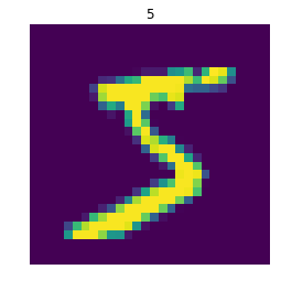
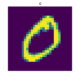
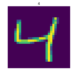
First we’ll load the training data, the MNIST digits/labels.

urlretrieve("http://deeplearning.net/data/mnist/mnist.pkl.gz", "mnist.pkl.gz")
with gzip.open("mnist.pkl.gz") as f:
    train_data, _, test_data = pickle.load(f, encoding="latin1")
train_data = list(train_data)
test_data = list(test_data)
for data in (train_data, test_data):
    one_hot = np.zeros((data[0].shape[0], 10))
    one_hot[np.arange(data[0].shape[0]), data[1]] = 1
    data[1] = one_hot

for i in range(3):
    plt.figure()
    plt.imshow(np.reshape(train_data[0][i], (28, 28)))
    plt.axis('off')
    plt.title(str(np.argmax(train_data[1][i])));

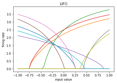
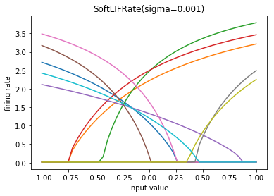
Recall that the plan is to construct the network using a differentiable approximation of spiking neurons. The spiking neuron model we’ll use is nengo.LIF, which has the differentiable approximation nengo_dl.SoftLIFRate. The parameters of nengo_dl.SoftLIFRate are the same as LIF/LIFRate, with the addition of the sigma parameter which controls the smoothness of the approximation (the lower the value of sigma, the closer SoftLIFRate approximates the true LIF/LIFRate firing curves.

Note: in reality MNIST is a simple enough task that we could just use nengo.LIFRate instead of nengo_dl.SoftLIFRate (we don’t need the additional smoothing from sigma). However, nengo_dl.SoftLIFRate is a useful thing to know about, and so we introduce it in this example.

# lif parameters
lif_neurons = nengo.LIF(amplitude=0.01)

# softlif parameters (lif parameters + sigma)
softlif_neurons = nengo_dl.SoftLIFRate(amplitude=0.01, sigma=0.001)

# ensemble parameters
ens_params = dict(max_rates=nengo.dists.Choice([100]), intercepts=nengo.dists.Choice([0]))

# plot some example LIF tuning curves
for neuron_type in (lif_neurons, softlif_neurons):
    with nengo.Network(seed=0) as net:
        ens = nengo.Ensemble(10, 1, neuron_type=neuron_type)

    with nengo_dl.Simulator(net) as sim:
        plt.figure()
        plt.plot(*nengo.utils.ensemble.tuning_curves(ens, sim))
        plt.xlabel("input value")
        plt.ylabel("firing rate")
        plt.title(str(neuron_type))

Build finished in 0:00:00
Optimization finished in 0:00:00
Construction finished in 0:00:00

/home/travis/build/nengo/nengo-dl/nengo_dl/simulator.py:126: UserWarning: No GPU support detected. It is recommended that you install tensorflow-gpu (`pip install tensorflow-gpu`).
  "No GPU support detected. It is recommended that you "

Build finished in 0:00:00
Optimization finished in 0:00:00
Construction finished in 0:00:00

We will use TensorNodes to construct the network, as they allow us to easily include features such as convolutional connections. To make things even easier, we’ll use nengo_dl.tensor_layer. This is a utility function for constructing TensorNodes that mimics the layer-based syntax of many deep learning packages (e.g. tf.layers). The full documentation for this function can be found here.

tensor_layer is used to build a sequence of layers, where each layer takes the output of the previous layer and applies some transformation to it. So when we build a tensor_layer we pass it the input to the layer, the transformation we want to apply (expressed as a function that accepts a tf.Tensor as input and produces a tf.Tensor as output), and any arguments to that transformation function. tensor_layer also has optional transform and synapse parameters that set those respective values on the Connection from the previous layer to the one being constructed.

Normally all signals in a Nengo model are (batched) vectors. However, certain layer functions, such as convolutional layers, may expect a different shape for their inputs. If the shape_in argument is specified for a tensor_layer then the inputs to the layer will automatically be reshaped to the given shape. Note that this shape does not include the batch dimension on the first axis, as that will be automatically set by the simulation.

tensor_layer can also be passed a Nengo NeuronType, instead of a Tensor function. In this case tensor_layer will construct an Ensemble implementing the given neuron nonlinearity (the rest of the arguments work the same).

Note that tensor_layer is just a syntactic wrapper for constructing TensorNodes or Ensembles; anything we build with a tensor_layer we could instead construct directly using those underlying components. tensor_layer just simplifies the construction of this common layer-based pattern.

def build_network(neuron_type, output_synapse=None):
    with nengo.Network() as net:
        # we'll make all the nengo objects in the network
        # non-trainable. we could train them if we wanted, but they don't
        # add any representational power so we can save some computation
        # by ignoring them. note that this doesn't affect the internal
        # components of tensornodes, which will always be trainable or
        # non-trainable depending on the code written in the tensornode.
        nengo_dl.configure_settings(trainable=False)

        # the input node that will be used to feed in input images
        inp = nengo.Node([0] * 28 * 28)

        # add the first convolutional layer
        x = nengo_dl.tensor_layer(
            inp, tf.layers.conv2d, shape_in=(28, 28, 1), filters=32,
            kernel_size=3)

        # apply the neural nonlinearity
        x = nengo_dl.tensor_layer(x, neuron_type, **ens_params)

        # add another convolutional layer
        x = nengo_dl.tensor_layer(
            x, tf.layers.conv2d, shape_in=(26, 26, 32),
            filters=64, kernel_size=3)
        x = nengo_dl.tensor_layer(x, neuron_type, **ens_params)

        # add a pooling layer
        x = nengo_dl.tensor_layer(
            x, tf.layers.average_pooling2d, shape_in=(24, 24, 64),
            pool_size=2, strides=2)

        # another convolutional layer
        x = nengo_dl.tensor_layer(
                x, tf.layers.conv2d, shape_in=(12, 12, 64),
                filters=128, kernel_size=3)
        x = nengo_dl.tensor_layer(x, neuron_type, **ens_params)

        # another pooling layer
        x = nengo_dl.tensor_layer(
            x, tf.layers.average_pooling2d, shape_in=(10, 10, 128),
            pool_size=2, strides=2)

        # linear readout
        x = nengo_dl.tensor_layer(x, tf.layers.dense, units=10)

        p = nengo.Probe(x, synapse=output_synapse)

    return net, inp, p

# construct the network
net, inp, out_p = build_network(softlif_neurons)

# construct the simulator
minibatch_size = 200
sim = nengo_dl.Simulator(net, minibatch_size=minibatch_size)

Build finished in 0:00:00
| #               Optimizing graph: creating signals                  | 0:00:00

/home/travis/build/nengo/nengo-dl/nengo_dl/simulator.py:126: UserWarning: No GPU support detected. It is recommended that you install tensorflow-gpu (`pip install tensorflow-gpu`).
  "No GPU support detected. It is recommended that you "

Optimization finished in 0:00:01
Construction finished in 0:00:02

Now we need to train this network to classify MNIST digits. First we load our input images and target labels.

# note that we need to add the time dimension (axis 1), which has length 1
# in this case. we're also going to reduce the number of test images, just to
# speed up this example.
train_inputs = {inp: train_data[0][:, None, :]}
train_targets = {out_p: train_data[1][:, None, :]}
test_inputs = {inp: test_data[0][:minibatch_size*2, None, :]}
test_targets = {out_p: test_data[1][:minibatch_size*2, None, :]}

Next we need to define our objective (error) function. Because this is a classification task we’ll use cross entropy, instead of the default mean squared error.

def objective(x, y):
    return tf.nn.softmax_cross_entropy_with_logits_v2(logits=x, labels=y)

The last thing we need to specify is the optimizer. For this example we’ll use RMSProp.

opt = tf.train.RMSPropOptimizer(learning_rate=0.001)

In order to quantify the network’s performance we will also define a classification error function (the percentage of test images classified incorrectly). We could use the cross entropy objective, but classification error is easier to interpret.

def classification_error(outputs, targets):
    return 100 * tf.reduce_mean(
        tf.cast(tf.not_equal(tf.argmax(outputs[:, -1], axis=-1),
                             tf.argmax(targets[:, -1], axis=-1)),
                tf.float32))

Now we are ready to train the network. In order to keep this example relatively quick we are going to download some pretrained weights. However, if you’d like to run the training yourself set do_training=True below.

print("error before training: %.2f%%" % sim.loss(test_inputs, test_targets,
                                                 classification_error))

do_training = False
if do_training:
    # run training
    sim.train(train_inputs, train_targets, opt, objective=objective, n_epochs=10)

    # save the parameters to file
    sim.save_params("./mnist_params")
else:
    # download pretrained weights
    urlretrieve(
        "https://drive.google.com/uc?export=download&id=1tNdnMPotIk8N0_rdv0XaL24dYqMGC2iM",
        "mnist_params.zip")
    with zipfile.ZipFile("mnist_params.zip") as f:
        f.extractall()

    # load parameters
    sim.load_params("./mnist_params")

print("error after training: %.2f%%" % sim.loss(test_inputs, test_targets,
                                                classification_error))

sim.close()

error before training: 89.00%
error after training: 0.75%

Now we want to change our network from SoftLIFRate to spiking LIF neurons. We rebuild our network with LIF neurons, and then load the saved parameters.

net, inp, out_p = build_network(lif_neurons, output_synapse=0.1)

sim = nengo_dl.Simulator(net, minibatch_size=minibatch_size, unroll_simulation=10)
sim.load_params("./mnist_params")

Build finished in 0:00:00
| #               Optimizing graph: creating signals                  | 0:00:00

/home/travis/build/nengo/nengo-dl/nengo_dl/simulator.py:126: UserWarning: No GPU support detected. It is recommended that you install tensorflow-gpu (`pip install tensorflow-gpu`).
  "No GPU support detected. It is recommended that you "

Optimization finished in 0:00:01
Construction finished in 0:00:03

To test our spiking network we need to run it for longer than one timestep, since we can only get an accurate measure of a spiking neuron’s output over time. So we’ll modify our test inputs so that they present the input image for 30 timesteps (0.03 seconds).

n_steps = 30
test_inputs_time = {inp: np.tile(v, (1, n_steps, 1)) for v in test_inputs.values()}
test_targets_time = {out_p: np.tile(v, (1, n_steps, 1)) for v in test_targets.values()}

print("spiking neuron error: %.2f%%" % sim.loss(test_inputs_time, test_targets_time,
                                                classification_error))

spiking neuron error: 1.00%

We can see that the spiking neural network is achieving similar accuracy as the network we trained with SoftLIFRate neurons. n_steps could be increased to further improve performance, since we would get a more accurate measure of each spiking neuron’s output.

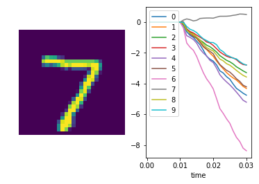
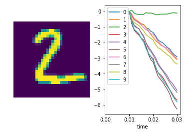
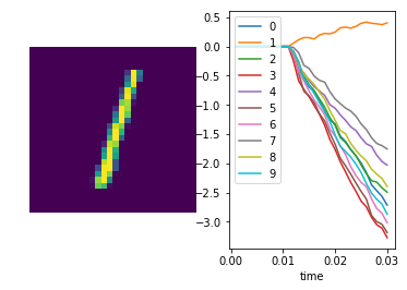
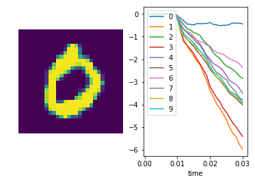
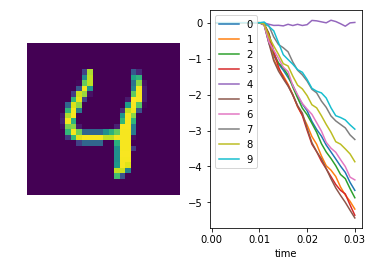
We can also plot some example outputs from the network, to see how it is performing over time.

sim.run_steps(n_steps, input_feeds={inp: test_inputs_time[inp][:minibatch_size]})

for i in range(5):
    plt.figure()
    plt.subplot(1, 2, 1)
    plt.imshow(np.reshape(test_data[0][i], (28, 28)))
    plt.axis('off')

    plt.subplot(1, 2, 2)
    plt.plot(sim.trange(), sim.data[out_p][i])
    plt.legend([str(i) for i in range(10)], loc="upper left")
    plt.xlabel("time")

Simulation finished in 0:01:03

sim.close()