Note

This documentation is for a development version. Click here for the latest stable release (v4.0.0).

Processes and how to use them

Processes in Nengo can be used to describe general functions or dynamical systems, including those with randomness. They can be useful if you want a Node output that has a state (like a dynamical system), and they’re also used for things like injecting noise into Ensembles so that you can not only have “white” noise that samples from a distribution, but can also have “colored” noise where subsequent samples are correlated with past samples.

This notebook will first present the basic process interface, then demonstrate some of the built-in Nengo processes and how they can be used in your code. It will also describe how to create your own custom process.

%matplotlib inline
import matplotlib.pyplot as plt
import numpy as np

import nengo

Interface

We will begin by looking at how to run an existing process instance.

The key functions for running processes are run, run_steps, and apply. The first two are for running without an input, and the third is for applying the process to an input.

There are also two helper functions, trange and ntrange, which return the time points corresponding to a process output, given either a length of time or a number of steps, respectively.

run: running a process for a length of time

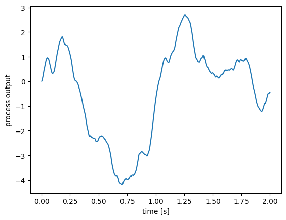
The run function runs a process for a given length of time, without any input. Many of the random processes in nengo.processes will be run this way, since they do not require an input signal.

# Create a process (details on the FilteredNoise process below)
process = nengo.processes.FilteredNoise(synapse=nengo.synapses.Alpha(0.1), seed=0)

# run the process for two seconds
y = process.run(2.0)

# get a corresponding two-second time range
t = process.trange(2.0)

plt.figure()
plt.plot(t, y)
plt.xlabel("time [s]")
plt.ylabel("process output")

Text(0, 0.5, 'process output')

run_steps: running a process for a number of steps

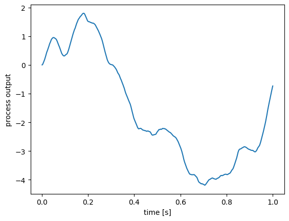
To run the process for a number of steps, use the run_steps function. The length of the generated signal will depend on the process’s default_dt.

process = nengo.processes.FilteredNoise(synapse=nengo.synapses.Alpha(0.1), seed=0)

# run the process for 1000 steps
y = process.run_steps(1000)

# get a corresponding 1000-step time range
t = process.ntrange(1000)

plt.figure()
plt.plot(t, y)
plt.xlabel("time [s]")
plt.ylabel("process output")

Text(0, 0.5, 'process output')

apply: running a process with an input

To run a process with an input, use the apply function.

process = nengo.synapses.Lowpass(0.2)

t = process.trange(5)
x = np.minimum(t % 2, 2 - (t % 2))  # sawtooth wave
y = process.apply(x)  # general to all Processes
z = process.filtfilt(x)  # specific to Synapses

plt.figure()
plt.plot(t, x, label="input")
plt.plot(t, y, label="output")
plt.plot(t, z, label="filtfilt")
plt.xlabel("time [s]")
plt.ylabel("signal")
plt.legend()

<matplotlib.legend.Legend at 0x7fce453912b0>

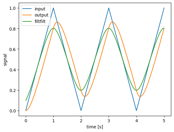
Note that Synapses are a special kind of process, and have the additional functions filt and filtfilt. filt works mostly the same as apply, but with some additional functionality such as the ability to filter along any axis. filtfilt provides zero-phase filtering.

Changing the time-step (dt and default_dt)

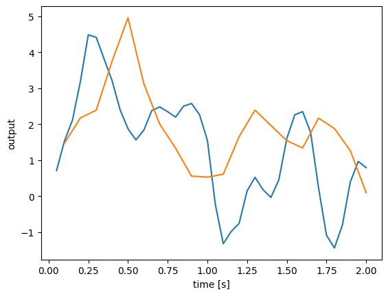
To run a process with a different time-step, you can either pass the new time step (dt) when calling the functions, or change the default_dt property of the process.

process = nengo.processes.FilteredNoise(synapse=nengo.synapses.Alpha(0.1), seed=0)
y1 = process.run(2.0, dt=0.05)
t1 = process.trange(2.0, dt=0.05)

process = nengo.processes.FilteredNoise(
    synapse=nengo.synapses.Alpha(0.1), default_dt=0.1, seed=0
)
y2 = process.run(2.0)
t2 = process.trange(2.0)

plt.figure()
plt.plot(t1, y1, label="dt = 0.05")
plt.plot(t2, y2, label="dt = 0.1")
plt.xlabel("time [s]")
plt.ylabel("output")

Text(0, 0.5, 'output')

WhiteSignal

The WhiteSignal process is used to generate band-limited white noise, with only frequencies below a given cutoff frequency.

with nengo.Network() as model:
    a = nengo.Node(nengo.processes.WhiteSignal(1.0, high=5, seed=0))
    b = nengo.Node(nengo.processes.WhiteSignal(1.0, high=10, seed=0))
    c = nengo.Node(nengo.processes.WhiteSignal(1.0, high=5, rms=0.3, seed=0))
    d = nengo.Node(nengo.processes.WhiteSignal(0.5, high=5, seed=0))
    ap = nengo.Probe(a)
    bp = nengo.Probe(b)
    cp = nengo.Probe(c)
    dp = nengo.Probe(d)

with nengo.Simulator(model) as sim:
    sim.run(1.0)

plt.figure()
plt.plot(sim.trange(), sim.data[ap], label="5 Hz cutoff")
plt.plot(sim.trange(), sim.data[bp], label="10 Hz cutoff")
plt.plot(sim.trange(), sim.data[cp], label="5 Hz cutoff, 0.3 RMS amplitude")
plt.plot(sim.trange(), sim.data[dp], label="5 Hz cutoff, 0.5 s period")
plt.xlabel("time [s]")
plt.legend(loc=2)

<matplotlib.legend.Legend at 0x7fce441ea970>

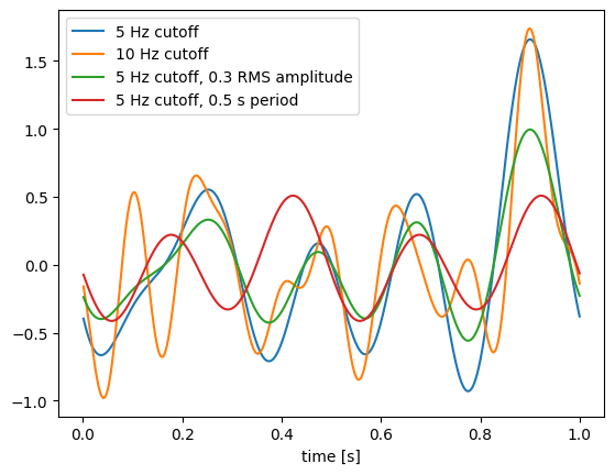
Note that the 10 Hz signal (green) has similar low frequency characteristics as the 5 Hz signal (blue), but with additional higher-frequency components. The 0.3 RMS amplitude 5 Hz signal (red) is the same as the original 5 Hz signal (blue), but scaled down (the default RMS amplitude is 0.5). Finally, the signal with a 0.5 s period (instead of a 1 s period like the others) is completely different, because changing the period changes the spacing of the random frequency components and thus creates a completely different signal. Note how the signal with the 0.5 s period repeats itself; for example, the value at \(t = 0\) is the same as the value at \(t = 0.5\), and the value at \(t = 0.4\) is the same as the value at \(t = 0.9\).

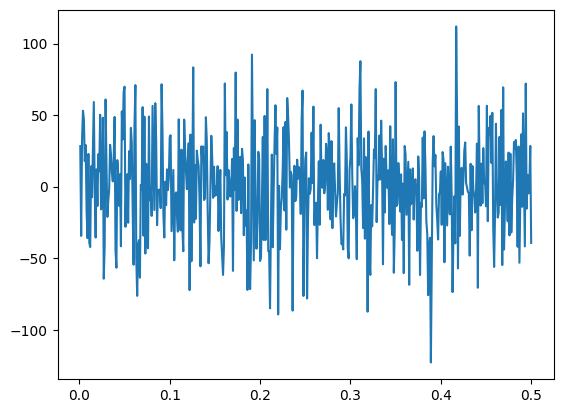
WhiteNoise

The WhiteNoise process generates white noise, with equal power across all frequencies. By default, it is scaled so that the integral process (Brownian noise) will have the same standard deviation regardless of dt.

process = nengo.processes.WhiteNoise(dist=nengo.dists.Gaussian(0, 1))

t = process.trange(0.5)
y = process.run(0.5)
plt.figure()
plt.plot(t, y)

[<matplotlib.lines.Line2D at 0x7fce4410e0a0>]

One use of the WhiteNoise process is to inject noise into neural populations. Here, we create two identical ensembles, but add a bit of noise to one and no noise to the other. We plot the membrane voltages of both.

process = nengo.processes.WhiteNoise(dist=nengo.dists.Gaussian(0, 0.01), seed=1)

with nengo.Network() as model:
    ens_args = {"encoders": [[1]], "intercepts": [0.01], "max_rates": [100]}
    a = nengo.Ensemble(1, 1, **ens_args)
    b = nengo.Ensemble(1, 1, noise=process, **ens_args)
    a_voltage = nengo.Probe(a.neurons, "voltage")
    b_voltage = nengo.Probe(b.neurons, "voltage")

with nengo.Simulator(model) as sim:
    sim.run(0.15)

plt.figure()
plt.plot(sim.trange(), sim.data[a_voltage], label="deterministic")
plt.plot(sim.trange(), sim.data[b_voltage], label="noisy")
plt.xlabel("time [s]")
plt.ylabel("voltage")
plt.legend(loc=4)

<matplotlib.legend.Legend at 0x7fce441c2fd0>

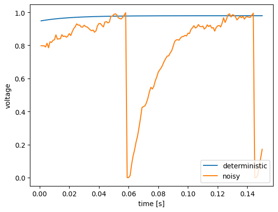
We see that the neuron without noise (blue) approaches its firing threshold, but never quite gets there. Adding a bit of noise (green) causes the neuron to occasionally jitter above the threshold, resulting in two spikes (where the voltage suddenly drops to zero).

FilteredNoise

The FilteredNoise process takes a white noise signal and passes it through a filter. Using any type of lowpass filter (e.g. Lowpass, Alpha) will result in a signal similar to WhiteSignal, but rather than being ideally filtered (i.e. no frequency content above the cutoff), the FilteredNoise signal will have some frequency content above the cutoff, with the amount depending on the filter used. Here, we can see how an Alpha filter (a second-order lowpass filter) is much better than the Lowpass filter (a first-order lowpass filter) at removing the high-frequency content.

process1 = nengo.processes.FilteredNoise(
    dist=nengo.dists.Gaussian(0, 0.01), synapse=nengo.Alpha(0.005), seed=0
)

process2 = nengo.processes.FilteredNoise(
    dist=nengo.dists.Gaussian(0, 0.01), synapse=nengo.Lowpass(0.005), seed=0
)

tlen = 0.5
plt.figure()
plt.plot(process1.trange(tlen), process1.run(tlen))
plt.plot(process2.trange(tlen), process2.run(tlen))

[<matplotlib.lines.Line2D at 0x7fce44053d90>]

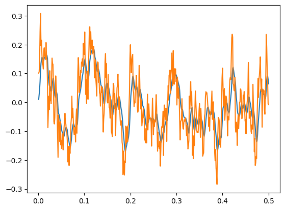
The FilteredNoise process with an Alpha synapse (blue) has significantly lower high-frequency components than a similar process with a Lowpass synapse (green).

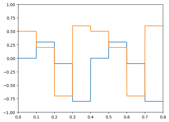
PresentInput

The PresentInput process is useful for presenting a series of static inputs to a network, where each input is shown for the same length of time. Once all the images have been shown, they repeat from the beginning. One application is presenting a series of images to a classification network.

inputs = [[0, 0.5], [0.3, 0.2], [-0.1, -0.7], [-0.8, 0.6]]
process = nengo.processes.PresentInput(inputs, presentation_time=0.1)

tlen = 0.8
plt.figure()
plt.plot(process.trange(tlen), process.run(tlen))
plt.xlim([0, tlen])
plt.ylim([-1, 1])

(-1.0, 1.0)

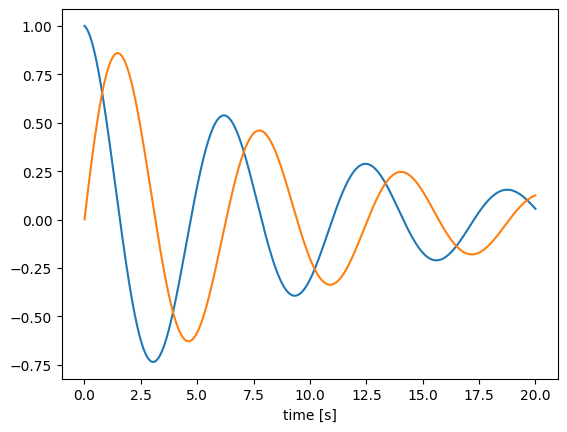
Custom processes

You can create custom processes by inheriting from the nengo.Process class and overloading the make_step and make_state methods.

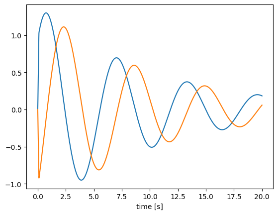
As an example, we’ll make a simple custom process that implements a two-dimensional oscillator dynamical system. The make_state function defines a state variable to store the state. The make_step function uses that state and a fixed A matrix to determine how the state changes over time.

One advantage to using a process over a simple function is that if we reset our simulator, make_step will be called again and the process state will be restored to the initial state.

class SimpleOscillator(nengo.Process):
    def make_state(self, shape_in, shape_out, dt, dtype=None):
        # return a dictionary mapping strings to their initial state
        return {"state": np.array([1.0, 0.0])}

    def make_step(self, shape_in, shape_out, dt, rng, state):
        A = np.array([[-0.1, -1.0], [1.0, -0.1]])
        s = state["state"]

        # define the step function, which will be called
        # by the node every time step
        def step(t):
            s[:] += dt * np.dot(A, s)
            return s

        return step  # return the step function


with nengo.Network() as model:
    a = nengo.Node(SimpleOscillator(), size_in=0, size_out=2)
    a_p = nengo.Probe(a)

with nengo.Simulator(model) as sim:
    sim.run(20.0)

plt.figure()
plt.plot(sim.trange(), sim.data[a_p])
plt.xlabel("time [s]")

Text(0.5, 0, 'time [s]')

We can generalize this process to one that can implement arbitrary linear dynamical systems, given A and B matrices. We will overload the __init__ method to take and store these matrices, as well as check the matrix shapes and set the default size in and out. The advantage of using the default sizes is that when we then create a node using the process, or run the process using apply, we do not need to specify the sizes.

class LTIProcess(nengo.Process):
    def __init__(self, A, B, **kwargs):
        A, B = np.asarray(A), np.asarray(B)

        # check that the matrix shapes are compatible
        assert A.ndim == 2 and A.shape[0] == A.shape[1]
        assert B.ndim == 2 and B.shape[0] == A.shape[0]

        # store the matrices for `make_step`
        self.A = A
        self.B = B

        # pass the default sizes to the Process constructor
        super().__init__(
            default_size_in=B.shape[1], default_size_out=A.shape[0], **kwargs
        )

    def make_state(self, shape_in, shape_out, dt, dtype=None):
        return {"state": np.zeros(self.A.shape[0])}

    def make_step(self, shape_in, shape_out, dt, rng, state):
        assert shape_in == (self.B.shape[1],)
        assert shape_out == (self.A.shape[0],)
        A, B = self.A, self.B
        s = state["state"]

        def step(t, x):
            s[:] += dt * (np.dot(A, s) + np.dot(B, x))
            return s

        return step


# demonstrate the LTIProcess in action
A = [[-0.1, -1], [1, -0.1]]
B = [[10], [-10]]

with nengo.Network() as model:
    u = nengo.Node(lambda t: 1 if t < 0.1 else 0)
    # we don't need to specify size_in and size_out!
    a = nengo.Node(LTIProcess(A, B))
    nengo.Connection(u, a)
    a_p = nengo.Probe(a)

with nengo.Simulator(model) as sim:
    sim.run(20.0)

plt.figure()
plt.plot(sim.trange(), sim.data[a_p])
plt.xlabel("time [s]")

Text(0.5, 0, 'time [s]')