Note

This documentation is for a development version. Click here for the latest stable release (v4.0.0).

2-dimensional representation

Ensembles of neurons represent information. In Nengo, we represent that information with real-valued vectors – lists of numbers. In this example, we will represent a two-dimensional vector with a single ensemble of leaky integrate-and-fire neurons.

Step 1: Create the network

Our model consists of a single ensemble, which we will call Neurons. It will represent a two-dimensional signal.

%matplotlib inline
import matplotlib.pyplot as plt
import numpy as np

import nengo

model = nengo.Network(label="2D Representation")
with model:
    # Our ensemble consists of 100 leaky integrate-and-fire neurons,
    # and represents a 2-dimensional signal
    neurons = nengo.Ensemble(100, dimensions=2)

Step 2: Provide input to the model

The signal that an ensemble represents varies over time. We will use a simple sine and cosine wave as examples of continuously changing signals.

with model:
    # Create input nodes representing the sine and cosine
    sin = nengo.Node(output=np.sin)
    cos = nengo.Node(output=np.cos)

Step 3: Connect the input to the ensemble

with model:
    # The indices in neurons define which dimension the input will project to
    nengo.Connection(sin, neurons[0])
    nengo.Connection(cos, neurons[1])

Step 4: Probe outputs

Anything that is probed will collect the data it produces over time, allowing us to analyze and visualize it later. Let’s collect all the data produced.

with model:
    sin_probe = nengo.Probe(sin, "output")
    cos_probe = nengo.Probe(cos, "output")
    neurons_probe = nengo.Probe(neurons, "decoded_output", synapse=0.01)

Step 5: Run the model

In order to run the model, we have to create a simulator. Then, we can run that simulator over and over again without affecting the original model.

with nengo.Simulator(model) as sim:
    sim.run(5)

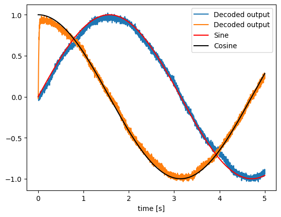
# Plot the decoded output of the ensemble
plt.figure()
plt.plot(sim.trange(), sim.data[neurons_probe], label="Decoded output")
plt.plot(sim.trange(), sim.data[sin_probe], "r", label="Sine")
plt.plot(sim.trange(), sim.data[cos_probe], "k", label="Cosine")
plt.legend()
plt.xlabel("time [s]")

Text(0.5, 0, 'time [s]')