Using the Izhikevich neuron model

The Izhikevich neuron model is a quadratic integrate-and-fire type model with a recovery variable. It is able to replicate several characteristics of biological neurons while remaining computationally efficient.

The Izhikevich neuron model is implemented in Nengo. To use it, use a nengo.Izhikevich instance as the neuron_type of an ensemble.

%matplotlib inline
import matplotlib.pyplot as plt
import numpy as np

import nengo
from nengo.utils.ensemble import tuning_curves
from nengo.utils.matplotlib import rasterplot

with nengo.Network(seed=0) as model:
    u = nengo.Node(lambda t: np.sin(2 * np.pi * t))
    ens = nengo.Ensemble(10, dimensions=1, neuron_type=nengo.Izhikevich())
    nengo.Connection(u, ens)

In addition to the usual decoded output and neural activity that can always be probed, you can probe the voltage and recovery terms of the Izhikevich model.

with model:
    out_p = nengo.Probe(ens, synapse=0.03)
    spikes_p = nengo.Probe(ens.neurons)
    voltage_p = nengo.Probe(ens.neurons, 'voltage')
    recovery_p = nengo.Probe(ens.neurons, 'recovery')

Simulating this model shows that we are able to decode a time-varying scalar with an ensemble of Izhikevich neurons.

with nengo.Simulator(model) as sim:
    sim.run(1.0)

t = sim.trange()
plt.figure(figsize=(12, 6))
plt.subplot(2, 1, 1)
plt.plot(t, sim.data[out_p])
plt.ylabel("Decoded output")
ax = plt.subplot(2, 1, 2)
rasterplot(t, sim.data[spikes_p], ax=ax)
plt.ylabel("Neuron");

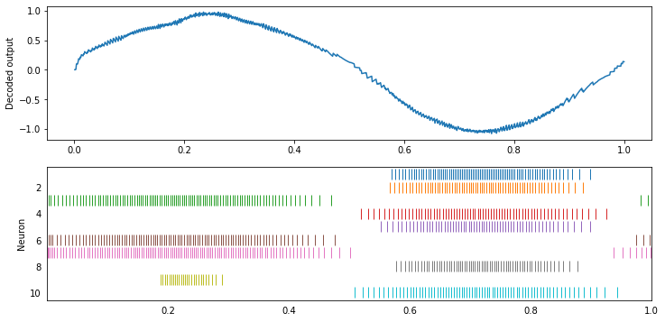
One thing you might notice is a slight bump in the decoded value at the start of the simulation. This occurs because of the adaptive nature of the Izhikevic model; it is easier to initiate the first spike than it is to ellicit further spikes.

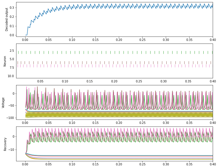
Let’s use a constant input and look at the first 100 ms of the simulation in more detail to see the difference between the first spike and subsequent spikes.

def izh_plot(sim):
    t = sim.trange()
    plt.figure(figsize=(12, 10))
    plt.subplot(4, 1, 1)
    plt.plot(t, sim.data[out_p])
    plt.ylabel("Decoded output")
    plt.xlim(right=t[-1])
    ax = plt.subplot(4, 1, 2)
    rasterplot(t, sim.data[spikes_p], ax=ax)
    plt.ylabel("Neuron")
    plt.xlim(right=t[-1])
    plt.subplot(4, 1, 3)
    plt.plot(t, sim.data[voltage_p])
    plt.ylabel("Voltage")
    plt.xlim(right=t[-1])
    plt.subplot(4, 1, 4)
    plt.plot(t, sim.data[recovery_p])
    plt.ylabel("Recovery")
    plt.xlim(right=t[-1])


u.output = 0.2
with nengo.Simulator(model) as sim:
    sim.run(0.1)
izh_plot(sim)

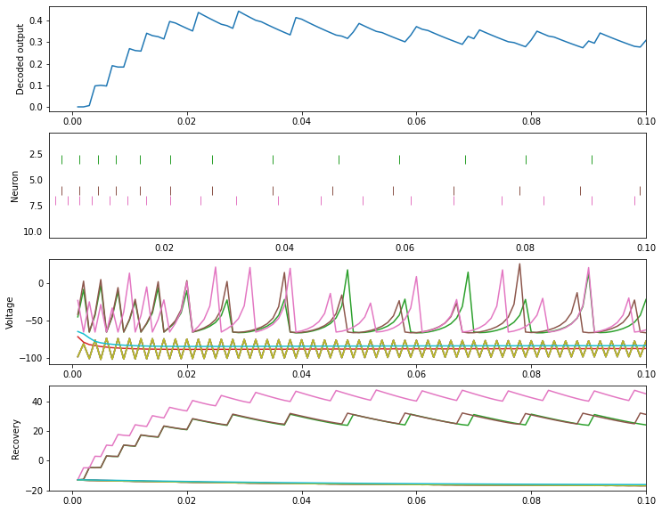
Those neurons that have an encoder of -1 receive negative current, and therefore remain at a low voltage.

Those neurons that have an encoder of 1 receive positive current, and start spiking rapidly. However, as they spike, the recovery variable grows, until it reaches a balance with the voltage such that the cells spike regularly.

This occurs because, by default, we use a set of parameters that models a “regular spiking” neuron. We can use parameters that model several different classes of neurons instead.

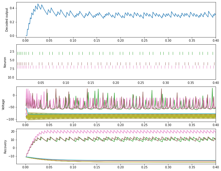
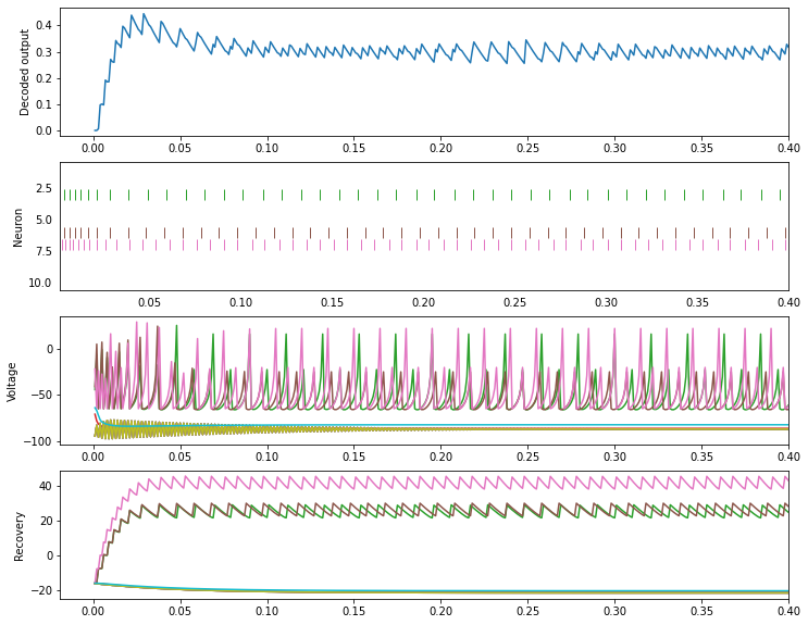
Intrinsically bursting (IB)

ens.neuron_type = nengo.Izhikevich(reset_voltage=-55, reset_recovery=4)
with nengo.Simulator(model) as sim:
    sim.run(0.4)
izh_plot(sim)

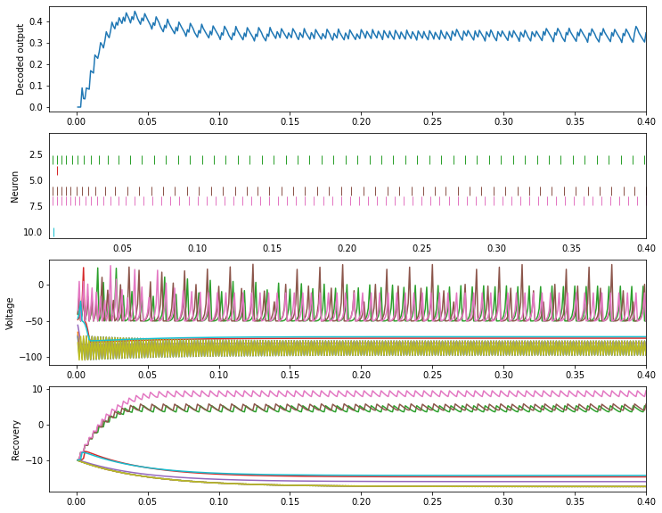
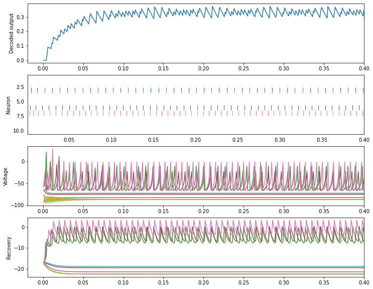
Chattering (CH)

ens.neuron_type = nengo.Izhikevich(reset_voltage=-50, reset_recovery=2)
with nengo.Simulator(model) as sim:
    sim.run(0.4)
izh_plot(sim)

Fast spiking (FS)

ens.neuron_type = nengo.Izhikevich(tau_recovery=0.1)
with nengo.Simulator(model) as sim:
    sim.run(0.4)
izh_plot(sim)

Low-threshold spiking (LTS)

ens.neuron_type = nengo.Izhikevich(coupling=0.25)
with nengo.Simulator(model) as sim:
    sim.run(0.4)
izh_plot(sim)

Resonator (RZ)

ens.neuron_type = nengo.Izhikevich(tau_recovery=0.1, coupling=0.26)
with nengo.Simulator(model) as sim:
    sim.run(0.4)
izh_plot(sim)

Caveats

Unfortunately, Izhikevich neurons can’t necessarily be used in all of the situations that LIFs are used, due to the more complex dynamics illustrated above.

The way that Nengo encodes and decodes information with neurons is informed by the tuning curves of those neurons. With Izhikevich neurons, the firing rate with a certain input current J changes; the spike rate is initially higher due to the adaptation illustrated above.

We try our best to generate tuning curves for Izhikevich neurons.

with nengo.Network(seed=0) as model:
    u = nengo.Node(lambda t: np.sin(2 * np.pi * t))
    ens = nengo.Ensemble(30, dimensions=1, neuron_type=nengo.Izhikevich())
    nengo.Connection(u, ens)
    out_p = nengo.Probe(ens, synapse=0.03)

with nengo.Simulator(model) as sim:
    plt.figure()
    plt.plot(*tuning_curves(ens, sim));

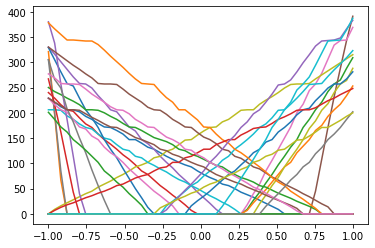
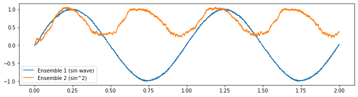
But these are not as accurate and clean as LIF curves, which is detrimental for function decoding.

u.output = lambda t: np.sin(2 * np.pi * t)
with model:
    square = nengo.Ensemble(30, dimensions=1, neuron_type=nengo.Izhikevich())
    nengo.Connection(ens, square, function=lambda x: x ** 2)
    square_p = nengo.Probe(square, synapse=0.03)

with nengo.Simulator(model) as sim:
    sim.run(2.0)

t = sim.trange()
plt.figure(figsize=(12, 3))
plt.plot(t, sim.data[out_p], label="Ensemble 1 (sin wave)")
plt.plot(t, sim.data[square_p], label="Ensemble 2 (sin^2)")
plt.legend(loc="best");

/mnt/d/Documents/nengo-repos/nengo/nengo/builder/optimizer.py:639: UserWarning: Skipping some optimization steps because SciPy is not installed. Installing SciPy may result in faster simulations.
  "Skipping some optimization steps because SciPy is "

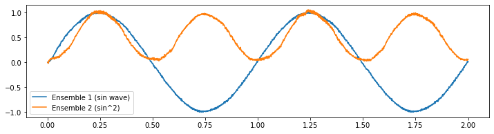
Some of these weird dynamics can be overcome by using Izhikevich neurons with different parameters.

square.neuron_type = nengo.Izhikevich(tau_recovery=0.2)

with nengo.Simulator(model) as sim:
    sim.run(2.0)

t = sim.trange()
plt.figure(figsize=(12, 3))
plt.plot(t, sim.data[out_p], label="Ensemble 1 (sin wave)")
plt.plot(t, sim.data[square_p], label="Ensemble 2 (sin^2)")
plt.legend(loc="best");

/mnt/d/Documents/nengo-repos/nengo/nengo/builder/optimizer.py:639: UserWarning: Skipping some optimization steps because SciPy is not installed. Installing SciPy may result in faster simulations.
  "Skipping some optimization steps because SciPy is "

Generally, however, Izhikevich neurons are most useful when trying to match known physiological properties of the system being modelled.