NEF summary
The Neural Engineering Framework (NEF) is one set of theoretical methods that are used in Nengo for constructing neural models. The NEF is based on Eliasmith & Anderson’s (2003) book from MIT Press. This notebook introduces the three main principles discussed in that book and implemented in Nengo.
[1]:
%matplotlib inline
import numpy as np
import matplotlib.pyplot as plt

import nengo
from nengo.dists import Uniform
from nengo.processes import WhiteSignal
from nengo.utils.ensemble import tuning_curves
from nengo.utils.ipython import hide_input
from nengo.utils.matplotlib import rasterplot


def aligned(n_neurons, radius=0.9):
    intercepts = np.linspace(-radius, radius, n_neurons)
    encoders = np.tile([[1], [-1]], (n_neurons // 2, 1))
    intercepts *= encoders[:, 0]
    return intercepts, encoders


hide_input()
[1]:
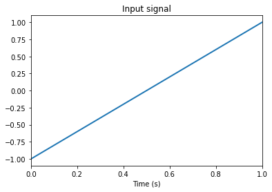
Principle 1: Representation
Encoding
Neural populations represent time-varying signals through their spiking responses. A signal is a vector of real numbers of arbitrary length. This example is a 1D signal going from -1 to 1 in 1 second.
[2]:
model = nengo.Network(label="NEF summary")
with model:
    input = nengo.Node(lambda t: t * 2 - 1)
    input_probe = nengo.Probe(input)
[3]:
with nengo.Simulator(model) as sim:
    sim.run(1.0)

plt.figure()
plt.plot(sim.trange(), sim.data[input_probe], lw=2)
plt.title("Input signal")
plt.xlabel("Time (s)")
plt.xlim(0, 1)
hide_input()
[3]:
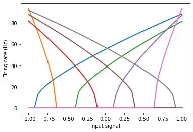
These signals drive neural populations based on each neuron’s tuning curve (which is similar to the current-frequency curve, if you’re familiar with that).
The tuning curve describes how much a particular neuron will fire as a function of the input signal.
[4]:
intercepts, encoders = aligned(8)  # Makes evenly spaced intercepts
with model:
    A = nengo.Ensemble(
        8,
        dimensions=1,
        intercepts=intercepts,
        max_rates=Uniform(80, 100),
        encoders=encoders,
    )
[5]:
with nengo.Simulator(model) as sim:
    eval_points, activities = tuning_curves(A, sim)

plt.figure()
plt.plot(eval_points, activities, lw=2)
plt.xlabel("Input signal")
plt.ylabel("Firing rate (Hz)")
hide_input()
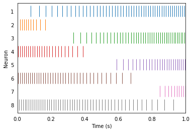
[5]:
We can drive these neurons with our input signal and observe their spiking activity over time.
[6]:
with model:
    nengo.Connection(input, A)
    A_spikes = nengo.Probe(A.neurons)
[7]:
with nengo.Simulator(model) as sim:
    sim.run(1)

plt.figure()
ax = plt.subplot(1, 1, 1)
rasterplot(sim.trange(), sim.data[A_spikes], ax)
ax.set_xlim(0, 1)
ax.set_ylabel("Neuron")
ax.set_xlabel("Time (s)")
hide_input()
[7]:
Decoding
We can estimate the input signal originally encoded by decoding the pattern of spikes. To do this, we first filter the spike train with a temporal filter that accounts for postsynaptic current (PSC) activity.
[8]:
model = nengo.Network(label="NEF summary")
with model:
    input = nengo.Node(lambda t: t * 2 - 1)
    input_probe = nengo.Probe(input)
    intercepts, encoders = aligned(8)  # Makes evenly spaced intercepts
    A = nengo.Ensemble(
        8,
        dimensions=1,
        intercepts=intercepts,
        max_rates=Uniform(80, 100),
        encoders=encoders,
    )
    nengo.Connection(input, A)
    A_spikes = nengo.Probe(A.neurons, synapse=0.01)
[9]:
with nengo.Simulator(model) as sim:
    sim.run(1)

scale = 180
plt.figure()
for i in range(A.n_neurons):
    plt.plot(sim.trange(), sim.data[A_spikes][:, i] - i * scale)
plt.xlim(0, 1)
plt.ylim(scale * (-A.n_neurons + 1), scale)
plt.ylabel("Neuron")
plt.yticks(
    np.arange(scale / 1.8, (-A.n_neurons + 1) * scale, -scale), np.arange(A.n_neurons)
)
hide_input()
[9]:
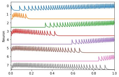
Then we mulitply those filtered spike trains with decoding weights and sum them together to give an estimate of the input based on the spikes.
The decoding weights are determined by minimizing the squared difference between the decoded estimate and the actual input signal.
[10]:
with model:
    A_probe = nengo.Probe(A, synapse=0.01)  # 10ms PSC filter
[11]:
with nengo.Simulator(model) as sim:
    sim.run(1)

plt.figure()
plt.plot(sim.trange(), sim.data[input_probe], label="Input signal")
plt.plot(sim.trange(), sim.data[A_probe], label="Decoded estimate")
plt.legend(loc="best")
plt.xlim(0, 1)
hide_input()
[11]:
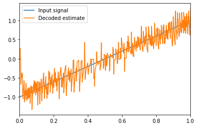
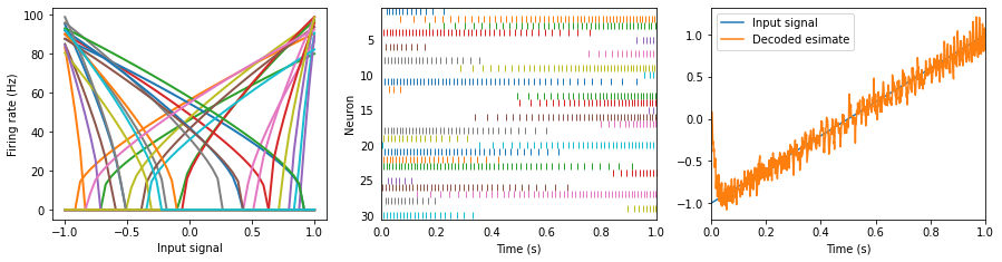
The accuracy of the decoded estimate increases as the number of neurons increases.
[12]:
model = nengo.Network(label="NEF summary")
with model:
    input = nengo.Node(lambda t: t * 2 - 1)
    input_probe = nengo.Probe(input)
    A = nengo.Ensemble(30, dimensions=1, max_rates=Uniform(80, 100))
    nengo.Connection(input, A)
    A_spikes = nengo.Probe(A.neurons)
    A_probe = nengo.Probe(A, synapse=0.01)
[13]:
with nengo.Simulator(model) as sim:
    sim.run(1)

plt.figure(figsize=(15, 3.5))

plt.subplot(1, 3, 1)
eval_points, activities = tuning_curves(A, sim)
plt.plot(eval_points, activities, lw=2)
plt.xlabel("Input signal")
plt.ylabel("Firing rate (Hz)")

ax = plt.subplot(1, 3, 2)
rasterplot(sim.trange(), sim.data[A_spikes], ax)
plt.xlim(0, 1)
plt.xlabel("Time (s)")
plt.ylabel("Neuron")

plt.subplot(1, 3, 3)
plt.plot(sim.trange(), sim.data[input_probe], label="Input signal")
plt.plot(sim.trange(), sim.data[A_probe], label="Decoded esimate")
plt.legend(loc="best")
plt.xlabel("Time (s)")
plt.xlim(0, 1)
hide_input()
[13]:
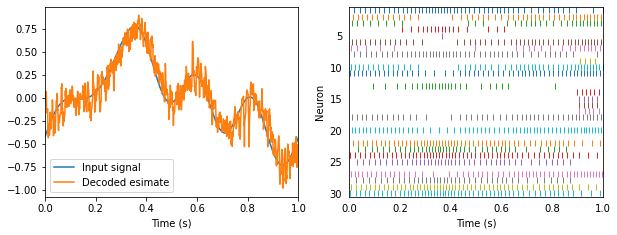
Any smooth signal can be encoded and decoded.
[14]:
model = nengo.Network(label="NEF summary")
with model:
    input = nengo.Node(WhiteSignal(1, high=5), size_out=1)
    input_probe = nengo.Probe(input)
    A = nengo.Ensemble(30, dimensions=1, max_rates=Uniform(80, 100))
    nengo.Connection(input, A)
    A_spikes = nengo.Probe(A.neurons)
    A_probe = nengo.Probe(A, synapse=0.01)
[15]:
with nengo.Simulator(model) as sim:
    sim.run(1)

plt.figure(figsize=(10, 3.5))
plt.subplot(1, 2, 1)
plt.plot(sim.trange(), sim.data[input_probe], label="Input signal")
plt.plot(sim.trange(), sim.data[A_probe], label="Decoded esimate")
plt.legend(loc="best")
plt.xlabel("Time (s)")
plt.xlim(0, 1)

ax = plt.subplot(1, 2, 2)
rasterplot(sim.trange(), sim.data[A_spikes], ax)
plt.xlim(0, 1)
plt.xlabel("Time (s)")
plt.ylabel("Neuron")
hide_input()
[15]:
Principle 2: Transformation
Encoding and decoding allow us to encode signals over time, and decode transformations of those signals.
In fact, we can decode arbitrary transformations of the input signal, not just the signal itself (as in the previous example).
Let’s decode the square of our white noise input.
[16]:
model = nengo.Network(label="NEF summary")
with model:
    input = nengo.Node(WhiteSignal(1, high=5), size_out=1)
    input_probe = nengo.Probe(input)
    A = nengo.Ensemble(30, dimensions=1, max_rates=Uniform(80, 100))
    Asquare = nengo.Node(size_in=1)
    nengo.Connection(input, A)
    nengo.Connection(A, Asquare, function=np.square)
    A_spikes = nengo.Probe(A.neurons)
    Asquare_probe = nengo.Probe(Asquare, synapse=0.01)
[17]:
with nengo.Simulator(model) as sim:
    sim.run(1)

plt.figure(figsize=(10, 3.5))
plt.subplot(1, 2, 1)
plt.plot(sim.trange(), sim.data[input_probe], label="Input signal")
plt.plot(sim.trange(), sim.data[Asquare_probe], label="Decoded esimate")
plt.plot(sim.trange(), np.square(sim.data[input_probe]), label="Input signal squared")
plt.legend(loc="best", fontsize="medium")
plt.xlabel("Time (s)")
plt.xlim(0, 1)

ax = plt.subplot(1, 2, 2)
rasterplot(sim.trange(), sim.data[A_spikes])
plt.xlim(0, 1)
plt.xlabel("Time (s)")
plt.ylabel("Neuron")
hide_input()
[17]:
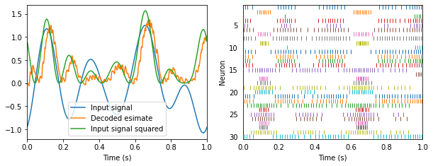
Notice that the spike trains are exactly the same. The only difference is how we’re interpreting those spikes. We told Nengo to compute a new set of decoders that estimate the function \(x^2\).
In general, the transformation principle determines how we can decode spike trains to compute linear and nonlinear transformations of signals encoded in a population of neurons. We can then project those transformed signals into another population, and repeat the process. Essentially, this provides a means of computing the neural connection weights to compute an arbitrary function between populations.
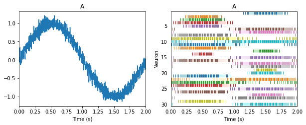
Suppose we are representing a sine wave.
[18]:
model = nengo.Network(label="NEF summary")
with model:
    input = nengo.Node(lambda t: np.sin(np.pi * t))
    A = nengo.Ensemble(30, dimensions=1, max_rates=Uniform(80, 100))
    nengo.Connection(input, A)
    A_spikes = nengo.Probe(A.neurons)
    A_probe = nengo.Probe(A, synapse=0.01)
[19]:
with nengo.Simulator(model) as sim:
    sim.run(2)

plt.figure(figsize=(10, 3.5))
plt.subplot(1, 2, 1)
plt.plot(sim.trange(), sim.data[A_probe])
plt.title("A")
plt.xlabel("Time (s)")
plt.xlim(0, 2)

ax = plt.subplot(1, 2, 2)
rasterplot(sim.trange(), sim.data[A_spikes], ax)
plt.xlim(0, 2)
plt.title("A")
plt.xlabel("Time (s)")
plt.ylabel("Neuron")
hide_input()
[19]:
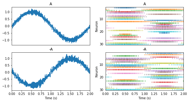
Linear transformations of that signal involve solving for the usual decoders, and scaling those decoding weights. Let us flip this sine wave upside down as it is transmitted between two populations (i.e. population A and population -A).
[20]:
with model:
    minusA = nengo.Ensemble(30, dimensions=1, max_rates=Uniform(80, 100))
    nengo.Connection(A, minusA, function=lambda x: -x)
    minusA_spikes = nengo.Probe(minusA.neurons)
    minusA_probe = nengo.Probe(minusA, synapse=0.01)
[21]:
with nengo.Simulator(model) as sim:
    sim.run(2)

plt.figure(figsize=(10, 5))
plt.subplot(2, 2, 1)
plt.plot(sim.trange(), sim.data[A_probe])
plt.title("A")
plt.xticks(())
plt.xlim(0, 2)

plt.subplot(2, 2, 3)
plt.plot(sim.trange(), sim.data[minusA_probe])
plt.title("-A")
plt.xlabel("Time (s)")
plt.xlim(0, 2)

ax = plt.subplot(2, 2, 2)
rasterplot(sim.trange(), sim.data[A_spikes], ax)
plt.xlim(0, 2)
plt.title("A")
plt.xticks(())
plt.ylabel("Neuron")

ax = plt.subplot(2, 2, 4)
rasterplot(sim.trange(), sim.data[minusA_spikes], ax)
plt.xlim(0, 2)
plt.title("-A")
plt.xlabel("Time (s)")
plt.ylabel("Neuron")
hide_input()
[21]:
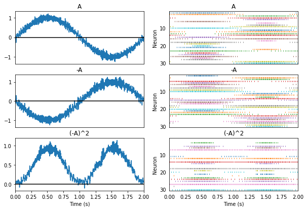
Nonlinear transformations involve solving for a new set of decoding weights. Let us add a third population connected to the second one and use it to compute \((-A)^2\).
[22]:
with model:
    A_squared = nengo.Ensemble(30, dimensions=1, max_rates=Uniform(80, 100))
    nengo.Connection(minusA, A_squared, function=lambda x: x ** 2)
    A_squared_spikes = nengo.Probe(A_squared.neurons)
    A_squared_probe = nengo.Probe(A_squared, synapse=0.02)
[23]:
with nengo.Simulator(model) as sim:
    sim.run(2)

plt.figure(figsize=(10, 6.5))
plt.subplot(3, 2, 1)
plt.plot(sim.trange(), sim.data[A_probe])
plt.axhline(0, color="k")
plt.title("A")
plt.xticks(())
plt.xlim(0, 2)

plt.subplot(3, 2, 3)
plt.plot(sim.trange(), sim.data[minusA_probe])
plt.axhline(0, color="k")
plt.title("-A")
plt.xticks(())
plt.xlim(0, 2)

plt.subplot(3, 2, 5)
plt.plot(sim.trange(), sim.data[A_squared_probe])
plt.axhline(0, color="k")
plt.title("(-A)^2")
plt.xlabel("Time (s)")
plt.xlim(0, 2)

ax = plt.subplot(3, 2, 2)
rasterplot(sim.trange(), sim.data[A_spikes], ax)
plt.xlim(0, 2)
plt.title("A")
plt.xticks(())
plt.ylabel("Neuron")

ax = plt.subplot(3, 2, 4)
rasterplot(sim.trange(), sim.data[minusA_spikes], ax)
plt.xlim(0, 2)
plt.title("-A")
plt.xticks(())
plt.ylabel("Neuron")

ax = plt.subplot(3, 2, 6)
rasterplot(sim.trange(), sim.data[A_squared_spikes], ax)
plt.xlim(0, 2)
plt.title("(-A)^2")
plt.xlabel("Time (s)")
plt.ylabel("Neuron")
hide_input()
[23]:
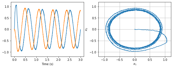
Principle 3: Dynamics
So far, we have been considering the values represented by ensembles as generic “signals.” However, if we think of them instead as state variables in a dynamical system, then we can apply the methods of control theory or dynamic systems theory to brain models. Nengo automatically translates from standard dynamical systems descriptions to descriptions consistent with neural dynamics.
In order to get interesting dynamics, we can connect populations recurrently (i.e., to themselves).
Below is a simple harmonic oscillator implemented using this third principle. It needs is a bit of input to get it started.
[24]:
model = nengo.Network(label="NEF summary")
with model:
    input = nengo.Node(lambda t: [1, 0] if t < 0.1 else [0, 0])
    oscillator = nengo.Ensemble(200, dimensions=2)
    nengo.Connection(input, oscillator)
    nengo.Connection(oscillator, oscillator, transform=[[1, 1], [-1, 1]], synapse=0.1)
    oscillator_probe = nengo.Probe(oscillator, synapse=0.02)
[25]:
with nengo.Simulator(model) as sim:
    sim.run(3)

plt.figure(figsize=(10, 3.5))
plt.subplot(1, 2, 1)
plt.plot(sim.trange(), sim.data[oscillator_probe])
plt.ylim(-1.2, 1.2)
plt.xlabel("Time (s)")

plt.subplot(1, 2, 2)
plt.plot(sim.data[oscillator_probe][:, 0], sim.data[oscillator_probe][:, 1])
plt.grid()
plt.axis([-1.2, 1.2, -1.2, 1.2])
plt.xlabel("$x_1$")
plt.ylabel("$x_2$")
hide_input()
[25]: