
Unsupervised learning
When we do error-modulated learning with the nengo.PES rule, we have a pretty clear idea of what we want to happen. Years of neuroscientific experiments have yielded learning rules explaining how synaptic strengths change given certain stimulation protocols. But what do these learning rules actually do to the information transmitted across an ensemble-to-ensemble connection?
We can investigate this in Nengo. Currently, we’ve implemented the nengo.BCM and nengo.Oja rules.
[1]:
import numpy as np
import matplotlib.pyplot as plt

%matplotlib inline

import nengo
[2]:
print(nengo.BCM.__doc__)
Bienenstock-Cooper-Munroe learning rule.

    Modifies connection weights as a function of the presynaptic activity
    and the difference between the postsynaptic activity and the average
    postsynaptic activity.

    Notes
    -----
    The BCM rule is dependent on pre and post neural activities,
    not decoded values, and so is not affected by changes in the
    size of pre and post ensembles. However, if you are decoding from
    the post ensemble, the BCM rule will have an increased effect on
    larger post ensembles because more connection weights are changing.
    In these cases, it may be advantageous to scale the learning rate
    on the BCM rule by ``1 / post.n_neurons``.

    Parameters
    ----------
    learning_rate : float, optional
        A scalar indicating the rate at which weights will be adjusted.
    pre_synapse : `.Synapse`, optional
        Synapse model used to filter the pre-synaptic activities.
    post_synapse : `.Synapse`, optional
        Synapse model used to filter the post-synaptic activities.
        If None, ``post_synapse`` will be the same as ``pre_synapse``.
    theta_synapse : `.Synapse`, optional
        Synapse model used to filter the theta signal.

    Attributes
    ----------
    learning_rate : float
        A scalar indicating the rate at which weights will be adjusted.
    post_synapse : `.Synapse`
        Synapse model used to filter the post-synaptic activities.
    pre_synapse : `.Synapse`
        Synapse model used to filter the pre-synaptic activities.
    theta_synapse : `.Synapse`
        Synapse model used to filter the theta signal.
[3]:
print(nengo.Oja.__doc__)
Oja learning rule.

    Modifies connection weights according to the Hebbian Oja rule, which
    augments typically Hebbian coactivity with a "forgetting" term that is
    proportional to the weight of the connection and the square of the
    postsynaptic activity.

    Notes
    -----
    The Oja rule is dependent on pre and post neural activities,
    not decoded values, and so is not affected by changes in the
    size of pre and post ensembles. However, if you are decoding from
    the post ensemble, the Oja rule will have an increased effect on
    larger post ensembles because more connection weights are changing.
    In these cases, it may be advantageous to scale the learning rate
    on the Oja rule by ``1 / post.n_neurons``.

    Parameters
    ----------
    learning_rate : float, optional
        A scalar indicating the rate at which weights will be adjusted.
    pre_synapse : `.Synapse`, optional
        Synapse model used to filter the pre-synaptic activities.
    post_synapse : `.Synapse`, optional
        Synapse model used to filter the post-synaptic activities.
        If None, ``post_synapse`` will be the same as ``pre_synapse``.
    beta : float, optional
        A scalar weight on the forgetting term.

    Attributes
    ----------
    beta : float
        A scalar weight on the forgetting term.
    learning_rate : float
        A scalar indicating the rate at which weights will be adjusted.
    post_synapse : `.Synapse`
        Synapse model used to filter the post-synaptic activities.
    pre_synapse : `.Synapse`
        Synapse model used to filter the pre-synaptic activities.
Step 1: Create a simple communication channel
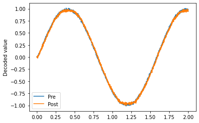
The only difference between this network and most models you’ve seen so far is that we’re going to set the decoder solver in the communication channel to generate a full connection weight matrix which we can then learn using typical delta learning rules.
[4]:
model = nengo.Network()
with model:
    sin = nengo.Node(lambda t: np.sin(t * 4))

    pre = nengo.Ensemble(100, dimensions=1)
    post = nengo.Ensemble(100, dimensions=1)

    nengo.Connection(sin, pre)
    conn = nengo.Connection(pre, post, solver=nengo.solvers.LstsqL2(weights=True))

    pre_p = nengo.Probe(pre, synapse=0.01)
    post_p = nengo.Probe(post, synapse=0.01)
[5]:
# Verify that it does a communication channel
with nengo.Simulator(model) as sim:
    sim.run(2.0)

plt.figure()
plt.plot(sim.trange(), sim.data[pre_p], label="Pre")
plt.plot(sim.trange(), sim.data[post_p], label="Post")
plt.ylabel("Decoded value")
plt.legend(loc="best")
[5]:
<matplotlib.legend.Legend at 0x7f9cc24147b8>
What does BCM do?
[6]:
conn.learning_rule_type = nengo.BCM(learning_rate=5e-10)
with model:
    weights_p = nengo.Probe(conn, "weights", synapse=0.01, sample_every=0.01)
[7]:
with nengo.Simulator(model) as sim:
    sim.run(20.0)
[8]:
plt.figure(figsize=(12, 8))
plt.subplot(2, 1, 1)
plt.plot(sim.trange(), sim.data[pre_p], label="Pre")
plt.plot(sim.trange(), sim.data[post_p], label="Post")
plt.ylabel("Decoded value")
plt.ylim(-1.6, 1.6)
plt.legend(loc="lower left")
plt.subplot(2, 1, 2)
# Find weight row with max variance
neuron = np.argmax(np.mean(np.var(sim.data[weights_p], axis=0), axis=1))
plt.plot(sim.trange(sample_every=0.01), sim.data[weights_p][..., neuron])
plt.ylabel("Connection weight")
[8]:
Text(0, 0.5, 'Connection weight')
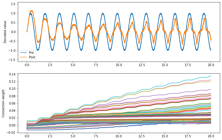
The BCM rule appears to cause the ensemble to either be on or off. This seems consistent with the idea that it potentiates active synapses, and depresses non-active synapses.
As well, we can show that BCM sparsifies the weights. The sparsity measure below uses the Gini measure of sparsity, for reasons explained in this paper.
[9]:
def sparsity_measure(vector):  # Gini index
    # Max sparsity = 1 (single 1 in the vector)
    v = np.sort(np.abs(vector))
    n = v.shape[0]
    k = np.arange(n) + 1
    l1norm = np.sum(v)
    summation = np.sum((v / l1norm) * ((n - k + 0.5) / n))
    return 1 - 2 * summation


print("Starting sparsity: {0}".format(sparsity_measure(sim.data[weights_p][0])))
print("Ending sparsity: {0}".format(sparsity_measure(sim.data[weights_p][-1])))
Starting sparsity: 0.20078881488763045
Ending sparsity: 0.4713694662392037
What does Oja do?
[10]:
conn.learning_rule_type = nengo.Oja(learning_rate=6e-8)
[11]:
with nengo.Simulator(model) as sim:
    sim.run(20.0)
[12]:
plt.figure(figsize=(12, 8))
plt.subplot(2, 1, 1)
plt.plot(sim.trange(), sim.data[pre_p], label="Pre")
plt.plot(sim.trange(), sim.data[post_p], label="Post")
plt.ylabel("Decoded value")
plt.ylim(-1.6, 1.6)
plt.legend(loc="lower left")
plt.subplot(2, 1, 2)
# Find weight row with max variance
neuron = np.argmax(np.mean(np.var(sim.data[weights_p], axis=0), axis=1))
plt.plot(sim.trange(sample_every=0.01), sim.data[weights_p][..., neuron])
plt.ylabel("Connection weight")
print("Starting sparsity: {0}".format(sparsity_measure(sim.data[weights_p][0])))
print("Ending sparsity: {0}".format(sparsity_measure(sim.data[weights_p][-1])))
Starting sparsity: 0.12587345437006392
Ending sparsity: 0.271998999392439
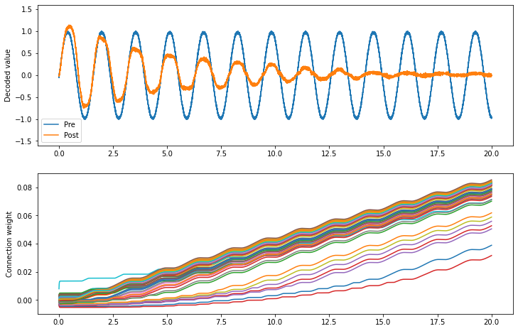
The Oja rule seems to attenuate the signal across the connection.
What do BCM and Oja together do?
We can apply both learning rules to the same connection by passing a list to learning_rule_type.
[13]:
conn.learning_rule_type = [
    nengo.BCM(learning_rate=5e-10),
    nengo.Oja(learning_rate=2e-9),
]
[14]:
with nengo.Simulator(model) as sim:
    sim.run(20.0)
[15]:
plt.figure(figsize=(12, 8))
plt.subplot(2, 1, 1)
plt.plot(sim.trange(), sim.data[pre_p], label="Pre")
plt.plot(sim.trange(), sim.data[post_p], label="Post")
plt.ylabel("Decoded value")
plt.ylim(-1.6, 1.6)
plt.legend(loc="lower left")
plt.subplot(2, 1, 2)
# Find weight row with max variance
neuron = np.argmax(np.mean(np.var(sim.data[weights_p], axis=0), axis=1))
plt.plot(sim.trange(sample_every=0.01), sim.data[weights_p][..., neuron])
plt.ylabel("Connection weight")
print("Starting sparsity: {0}".format(sparsity_measure(sim.data[weights_p][0])))
print("Ending sparsity: {0}".format(sparsity_measure(sim.data[weights_p][-1])))
Starting sparsity: 0.14215843751813528
Ending sparsity: 0.4464210578392487
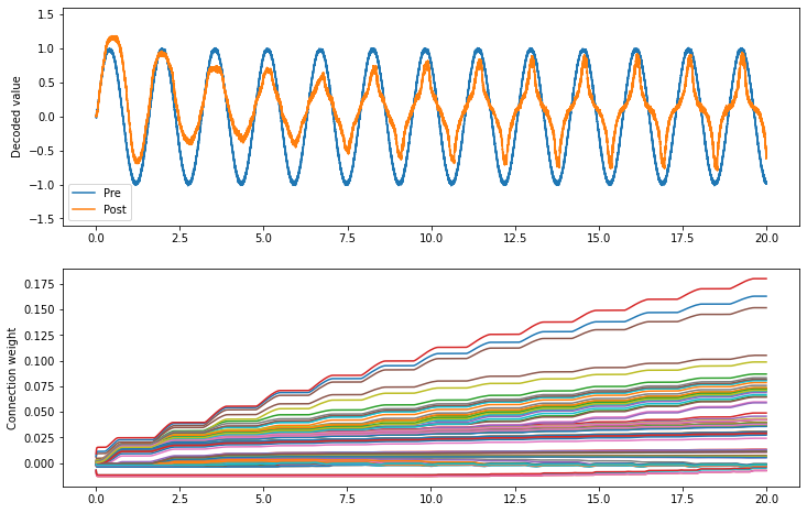
The combination of the two appears to accentuate the on-off nature of the BCM rule. As the Oja rule enforces a soft upper or lower bound for the connection weight, the combination of both rules may be more stable than BCM alone.
That’s mostly conjecture, however; a thorough investigation of the BCM and Oja rules and how they interact has not yet been done.