Tuning curves
One of the most common ways to tweak models and debug failures is to look at the tuning curves of the neurons in an ensemble. The tuning curve tells us how each neuron responds to an incoming input signal.
1-dimensional ensembles
The tuning curve is easiest to interpret in the one-dimensional case. Since the input is a single scalar, we use that value as the x-axis, and the neuron response as the y-axis.
[1]:
%matplotlib inline
import numpy as np
import matplotlib.pyplot as plt
from mpl_toolkits.mplot3d import Axes3D

import nengo
from nengo.dists import Choice
from nengo.utils.ensemble import response_curves, tuning_curves
[2]:
model = nengo.Network()
with model:
    ens_1d = nengo.Ensemble(15, dimensions=1)
with nengo.Simulator(model) as sim:
    eval_points, activities = tuning_curves(ens_1d, sim)

plt.figure()
plt.plot(eval_points, activities)
# We could have alternatively shortened this to
# plt.plot(*tuning_curves(ens_1d, sim))
plt.ylabel("Firing rate (Hz)")
plt.xlabel("Input scalar, x")
[2]:
Text(0.5, 0, 'Input scalar, x')
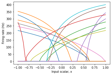
Each coloured line represents the response on one neuron. As you can see, the neurons cover the space pretty well, but there is no clear pattern to their responses.
If there is some biological or functional reason to impose some pattern to their responses, we can do so by changing the parameters of the ensemble.
[3]:
ens_1d.intercepts = Choice([-0.2])  # All neurons have x-intercept -0.2
with nengo.Simulator(model) as sim:
    plt.figure()
    plt.plot(*tuning_curves(ens_1d, sim))

plt.ylabel("Firing rate (Hz)")
plt.xlabel("Input scalar, x")
[3]:
Text(0.5, 0, 'Input scalar, x')
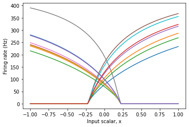
Now, there is a clear pattern to the tuning curve. However, note that some neurons start firing at -0.2, while others stop firing at 0.2. This is because the input signal, x, is multiplied by a neuron’s encoder when it is converted to input current.
We could further constrain the tuning curves by changing the encoders of the ensemble.
[4]:
ens_1d.encoders = Choice([[1]])  # All neurons have encoder [1]
with nengo.Simulator(model) as sim:
    plt.figure()
    plt.plot(*tuning_curves(ens_1d, sim))

plt.ylabel("Firing rate (Hz)")
plt.xlabel("Input scalar, x")
[4]:
Text(0.5, 0, 'Input scalar, x')
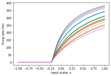
This gives us an ensemble of neurons that respond very predictably to input. In some cases, this is important to the proper functioning of a model, or to matching what we know about the physiology of a brain area or neuron type.
2-dimensional ensembles
In a two-dimensional ensemble, the input is represented by two scalar values, meaning that we will need three axes to represent its tuning curve; two for input dimensions, and one for the neural activity.
Fortunately, we are able to plot data in 3D.
If there is a clear pattern to the tuning curves, then visualizing them all is (sort of) possible.
[5]:
model = nengo.Network()
with model:
    ens_2d = nengo.Ensemble(15, dimensions=2, encoders=Choice([[1, 1]]))
with nengo.Simulator(model) as sim:
    eval_points, activities = tuning_curves(ens_2d, sim)

plt.figure(figsize=(8, 8))
ax = plt.subplot(111, projection="3d")
ax.set_title("Tuning curve of all neurons")
for i in range(ens_2d.n_neurons):
    ax.plot_surface(
        eval_points.T[0], eval_points.T[1], activities.T[i], cmap=plt.cm.autumn
    )
ax.set_xlabel("$x_1$")
ax.set_ylabel("$x_2$")
ax.set_zlabel("Firing rate (Hz)")
[5]:
Text(0.5, 0, 'Firing rate (Hz)')
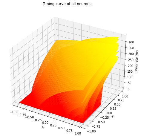
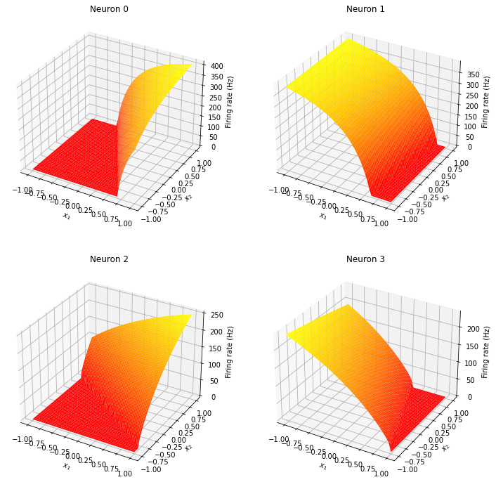
But in most cases, for 2D ensembles, we have to look at each neuron’s tuning curve separately.
[6]:
ens_2d.encoders = nengo.Default
with nengo.Simulator(model) as sim:
    eval_points, activities = tuning_curves(ens_2d, sim)

plt.figure(figsize=(12, 12))
for i in range(4):
    ax = plt.subplot(2, 2, i + 1, projection=Axes3D.name)
    ax.set_title("Neuron %d" % i)
    ax.plot_surface(
        eval_points.T[0], eval_points.T[1], activities.T[i], cmap=plt.cm.autumn
    )
    ax.set_xlabel("$x_1$")
    ax.set_ylabel("$x_2$")
    ax.set_zlabel("Firing rate (Hz)")
N-dimensional ensembles
The tuning_curve function accepts ensembles of any dimensionality, and will always return eval_points and activities. However, for ensembles of dimensionality greater than 2, these are large arrays and it becomes nearly impossible to visualize them.
There are two main approaches to investigating the tuning curves of ensembles of arbitrary dimensionality.
Clamp some axes
In many cases, we only care about the neural sensitivity to one or two dimensions. We can investigate those dimensions specifically by only varying those dimensions, and keeping the rest constant.
To do this, we will use the inputs argument to the tuning_curves function, which allows us to define the input signals that will drive the neurons to determine their activity. In other words, we are specifying the eval_point parameter to generate the activities.
[7]:
model = nengo.Network()
with model:
    ens_3d = nengo.Ensemble(15, dimensions=3)

inputs = np.zeros((50, 3))
# Vary the first dimension
inputs[:, 0] = np.linspace(-ens_3d.radius, ens_3d.radius, 50)
inputs[:, 1] = 0.5  # Clamp the second dimension
inputs[:, 2] = 0.5  # Clamp the third dimension

with nengo.Simulator(model) as sim:
    eval_points, activities = tuning_curves(ens_3d, sim, inputs=inputs)

assert eval_points is inputs  # The inputs will be returned as eval_points

plt.figure()
plt.plot(inputs.T[0], activities)
plt.ylabel("Firing rate (Hz)")
plt.xlabel("$x_0$")
[7]:
Text(0.5, 0, '$x_0$')
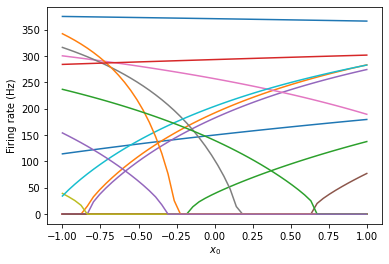
Notice that these tuning curves are much more broad than those in the 1-dimensional case. This is because some neurons are not very sensitive to the dimension that are varying, and are instead sensitive to one or two of the other dimensions. If we wanted these neurons to be more sharply tuned to this dimension, we could change their encoders to be more tuned to this dimension.
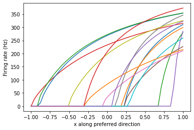
Response curves
If all else fails, we can still get some information about the tuning properties of the neurons in the ensemble using the response curve. The response curve is similar to the tuning curve, but instead of looking at the neural response to a particular input stimulus, we are instead looking at its response to (relative) injected current. This is analogous to the tuning curves with the inputs aligned to the preferred directions of each neuron.
[8]:
model = nengo.Network()
with model:
    ens_5d = nengo.Ensemble(15, dimensions=5)
with nengo.Simulator(model) as sim:
    plt.figure()
    plt.plot(*response_curves(ens_5d, sim))

plt.ylabel("Firing rate (Hz)")
plt.xlabel("x along preferred direction")
[8]:
Text(0.5, 0, 'x along preferred direction')