Controlled oscillator

The controlled oscillator is an oscillator with an extra input that controls the frequency of the oscillation.

To implement a basic oscillator, we would use a neural ensemble of two dimensions that has the following dynamics:

\[\begin{split}\dot{x} = \begin{bmatrix} 0 && - \omega \\ \omega && 0 \end{bmatrix} x\end{split}\]

where the frequency of oscillation is \(\omega \over {2 \pi}\) Hz.

We need the neurons to represent three variables, \(x_0\), \(x_1\), and \(\omega\). According the the dynamics principle of the NEF, in order to implement some particular dynamics, we need to convert this dynamics equation into a feedback function:

\[\begin{split}\begin{align} \dot{x} &= f(x) \\ &\implies f_{feedback}(x) = x + \tau f(x) \end{align}\end{split}\]

where \(\tau\) is the post-synaptic time constant of the feedback connection.

In this case, the feedback function to be computed is

\[\begin{split}\begin{align} f_{feedback}(x) &= x + \tau \begin{bmatrix} 0 && - \omega \\ \omega && 0 \end{bmatrix} x \\ &= \begin{bmatrix} x_0 - \tau \cdot \omega \cdot x_1 \\ x_1 + \tau \cdot \omega \cdot x_0 \end{bmatrix} \end{align}\end{split}\]

Since the neural ensemble represents all three variables but the dynamics only affects the first two (\(x_0\), \(x_1\)), we need the feedback function to not affect that last variable. We do this by adding a zero to the feedback function.

\[\begin{split}f_{feedback}(x) = \begin{bmatrix} x_0 - \tau \cdot \omega \cdot x_1 \\ x_1 + \tau \cdot \omega \cdot x_0 \\ 0 \end{bmatrix}\end{split}\]

We also generally want to keep the ranges of variables represented within an ensemble to be approximately the same. In this case, if \(x_0\) and \(x_1\) are between -1 and 1, \(\omega\) will also be between -1 and 1, giving a frequency range of \(-1 \over {2 \pi}\) to \(1 \over {2 \pi}\). To increase this range, we introduce a scaling factor to \(\omega\) called \(\omega_{max}\).

\[\begin{split}f_{feedback}(x) = \begin{bmatrix} x_0 - \tau \cdot \omega \cdot \omega_{max} \cdot x_1 \\ x_1 + \tau \cdot \omega \cdot \omega_{max} \cdot x_0 \\ 0 \end{bmatrix}\end{split}\]

%matplotlib inline
import matplotlib.pyplot as plt

import nengo
from nengo.processes import Piecewise

Step 1: Create the network

tau = 0.1  # Post-synaptic time constant for feedback
w_max = 10  # Maximum frequency in Hz is w_max/(2*pi)

model = nengo.Network(label="Controlled Oscillator")
with model:
    # The ensemble for the oscillator
    oscillator = nengo.Ensemble(500, dimensions=3, radius=1.7)

    # The feedback connection
    def feedback(x):
        x0, x1, w = x  # These are the three variables stored in the ensemble
        return x0 - w * w_max * tau * x1, x1 + w * w_max * tau * x0, 0

    nengo.Connection(oscillator, oscillator, function=feedback, synapse=tau)

    # The ensemble for controlling the speed of oscillation
    frequency = nengo.Ensemble(100, dimensions=1)

    nengo.Connection(frequency, oscillator[2])

Step 2: Create the input

with model:
    # We need a quick input at the beginning to start the oscillator
    initial = nengo.Node(Piecewise({0: [1, 0, 0], 0.15: [0, 0, 0]}))
    nengo.Connection(initial, oscillator)

    # Vary the speed over time
    input_frequency = nengo.Node(Piecewise({0: 1, 1: 0.5, 2: 0, 3: -0.5, 4: -1}))

    nengo.Connection(input_frequency, frequency)

Step 3: Add Probes

with model:
    # Indicate which values to record
    oscillator_probe = nengo.Probe(oscillator, synapse=0.03)

Step 4: Run the Model

with nengo.Simulator(model) as sim:
    sim.run(5)

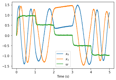
Step 5: Plot the Results

plt.figure()
plt.plot(sim.trange(), sim.data[oscillator_probe])
plt.xlabel("Time (s)")
plt.legend(["$x_0$", "$x_1$", r"$\omega$"])

<matplotlib.legend.Legend at 0x7fa449ded160>