Classifying Fashion MNIST with spiking activations
In this example we assume that you are already familiar with building and training standard, non-spiking neural networks in PyTorch. We would recommend checking out the PyTorch documentation if you would like a more basic introduction to how PyTorch works. In this example we will walk through how we can convert a non-spiking model into a spiking model using PyTorchSpiking, and various techniques that can be used to fine tune performance.
[1]:
# pylint: disable=redefined-outer-name

import matplotlib.pyplot as plt
import numpy as np
import torch
import torchvision

import pytorch_spiking

torch.manual_seed(0)
np.random.seed(0)
Loading data
We’ll begin by loading the Fashion MNIST data:
[2]:
train_images, train_labels = zip(
    *torchvision.datasets.FashionMNIST(".", train=True, download=True)
)
train_images = np.asarray([np.array(img) for img in train_images], dtype=np.float32)
train_labels = np.asarray(train_labels, dtype=np.int64)
test_images, test_labels = zip(
    *torchvision.datasets.FashionMNIST(".", train=False, download=True)
)
test_images = np.asarray([np.array(img) for img in train_images], dtype=np.float32)
test_labels = np.asarray(train_labels, dtype=np.int64)

# normalize images so values are between 0 and 1
train_images = train_images / 255.0
test_images = test_images / 255.0

class_names = [
    "T-shirt/top",
    "Trouser",
    "Pullover",
    "Dress",
    "Coat",
    "Sandal",
    "Shirt",
    "Sneaker",
    "Bag",
    "Ankle boot",
]
num_classes = len(class_names)

plt.figure(figsize=(10, 10))
for i in range(25):
    plt.subplot(5, 5, i + 1)
    plt.imshow(train_images[i], cmap=plt.cm.binary)
    plt.axis("off")
    plt.title(class_names[train_labels[i]])
Downloading http://fashion-mnist.s3-website.eu-central-1.amazonaws.com/train-images-idx3-ubyte.gz
Downloading http://fashion-mnist.s3-website.eu-central-1.amazonaws.com/train-images-idx3-ubyte.gz to ./FashionMNIST/raw/train-images-idx3-ubyte.gz
100.0%
Extracting ./FashionMNIST/raw/train-images-idx3-ubyte.gz to ./FashionMNIST/raw

Downloading http://fashion-mnist.s3-website.eu-central-1.amazonaws.com/train-labels-idx1-ubyte.gz
Downloading http://fashion-mnist.s3-website.eu-central-1.amazonaws.com/train-labels-idx1-ubyte.gz to ./FashionMNIST/raw/train-labels-idx1-ubyte.gz
100.0%
Extracting ./FashionMNIST/raw/train-labels-idx1-ubyte.gz to ./FashionMNIST/raw

Downloading http://fashion-mnist.s3-website.eu-central-1.amazonaws.com/t10k-images-idx3-ubyte.gz
Downloading http://fashion-mnist.s3-website.eu-central-1.amazonaws.com/t10k-images-idx3-ubyte.gz to ./FashionMNIST/raw/t10k-images-idx3-ubyte.gz
100.0%
Extracting ./FashionMNIST/raw/t10k-images-idx3-ubyte.gz to ./FashionMNIST/raw

Downloading http://fashion-mnist.s3-website.eu-central-1.amazonaws.com/t10k-labels-idx1-ubyte.gz
Downloading http://fashion-mnist.s3-website.eu-central-1.amazonaws.com/t10k-labels-idx1-ubyte.gz to ./FashionMNIST/raw/t10k-labels-idx1-ubyte.gz
100.0%
Extracting ./FashionMNIST/raw/t10k-labels-idx1-ubyte.gz to ./FashionMNIST/raw

Non-spiking model
Next we’ll build and train a simple non-spiking model to classify the Fashion MNIST images.
[3]:
model = torch.nn.Sequential(
    torch.nn.Linear(784, 128),
    torch.nn.ReLU(),
    torch.nn.Linear(128, 10),
)


def train(input_model, train_x, test_x):
    minibatch_size = 32
    optimizer = torch.optim.Adam(input_model.parameters())

    input_model.train()
    for j in range(10):
        train_acc = 0
        for i in range(train_x.shape[0] // minibatch_size):
            input_model.zero_grad()

            batch_in = train_x[i * minibatch_size : (i + 1) * minibatch_size]
            # flatten images
            batch_in = batch_in.reshape((-1,) + train_x.shape[1:-2] + (784,))
            batch_label = train_labels[i * minibatch_size : (i + 1) * minibatch_size]
            output = input_model(torch.tensor(batch_in))

            # compute sparse categorical cross entropy loss
            logp = torch.nn.functional.log_softmax(output, dim=-1)
            logpy = torch.gather(logp, 1, torch.tensor(batch_label).view(-1, 1))
            loss = -logpy.mean()

            loss.backward()
            optimizer.step()

            train_acc += torch.mean(
                torch.eq(torch.argmax(output, dim=1), torch.tensor(batch_label)).float()
            )

        train_acc /= i + 1
        print(f"Train accuracy ({j}): {train_acc.numpy()}")

    # compute test accuracy
    input_model.eval()
    test_acc = 0
    for i in range(test_x.shape[0] // minibatch_size):
        batch_in = test_x[i * minibatch_size : (i + 1) * minibatch_size]
        batch_in = batch_in.reshape((-1,) + test_x.shape[1:-2] + (784,))
        batch_label = test_labels[i * minibatch_size : (i + 1) * minibatch_size]
        output = input_model(torch.tensor(batch_in))

        test_acc += torch.mean(
            torch.eq(torch.argmax(output, dim=1), torch.tensor(batch_label)).float()
        )

    test_acc /= i + 1

    print(f"Test accuracy: {test_acc.numpy()}")


train(model, train_images, test_images)
Train accuracy (0): 0.8192166686058044
Train accuracy (1): 0.8625666499137878
Train accuracy (2): 0.8756499886512756
Train accuracy (3): 0.883983314037323
Train accuracy (4): 0.8913666605949402
Train accuracy (5): 0.8968999981880188
Train accuracy (6): 0.9005166888237
Train accuracy (7): 0.9055166840553284
Train accuracy (8): 0.9081166386604309
Train accuracy (9): 0.9118833541870117
Test accuracy: 0.9060333371162415
Spiking model
Next we will create an equivalent spiking model. There are three important changes here:
Add a temporal dimension to the data/model.
Spiking models always run over time (i.e., each forward pass through the model will run for some number of timesteps). This means that we need to add a temporal dimension to the data, so instead of having shape (batch_size, ...) it will have shape (batch_size, n_steps, ...). For those familiar with working with RNNs, the principles are the same; a spiking neuron accepts temporal data and computes over time, just like an RNN.
Replace any activation functions with
pytorch_spiking.SpikingActivation.
pytorch_spiking.SpikingActivation can encapsulate any activation function, and will produce an equivalent spiking implementation. Neurons will spike at a rate proportional to the output of the base activation function. For example, if the activation function is outputting a value of 10, then the wrapped SpikingActivation will output spikes at a rate of 10Hz (i.e., 10 spikes per 1 simulated second, where 1 simulated second is equivalent to some number of timesteps, determined by the
dt parameter of SpikingActivation).
Pool across time
The output of our pytorch_spiking.SpikingActivation layer is also a timeseries. For classification, we need to aggregate that temporal information somehow to generate a final prediction. Averaging the output over time is usually a good approach (but not the only method; we could also, e.g., look at the output on the last timestep or the time to first spike). We add a pytorch_spiking.TemporalAvgPool layer to average across the temporal dimension of the data.
[4]:
# repeat the images for n_steps
n_steps = 10
train_sequences = np.tile(train_images[:, None], (1, n_steps, 1, 1))
test_sequences = np.tile(test_images[:, None], (1, n_steps, 1, 1))
[5]:
spiking_model = torch.nn.Sequential(
    torch.nn.Linear(784, 128),
    # wrap ReLU in SpikingActivation
    pytorch_spiking.SpikingActivation(torch.nn.ReLU(), spiking_aware_training=False),
    # use average pooling layer to average spiking output over time
    pytorch_spiking.TemporalAvgPool(),
    torch.nn.Linear(128, 10),
)

# train the model, identically to the non-spiking version,
# except using the time sequences as input
train(spiking_model, train_sequences, test_sequences)
Train accuracy (0): 0.8192333579063416
Train accuracy (1): 0.8624833226203918
Train accuracy (2): 0.8749499917030334
Train accuracy (3): 0.8830000162124634
Train accuracy (4): 0.8889166712760925
Train accuracy (5): 0.8942833542823792
Train accuracy (6): 0.8995000123977661
Train accuracy (7): 0.9032333493232727
Train accuracy (8): 0.9077666401863098
Train accuracy (9): 0.9107499718666077
Test accuracy: 0.17543333768844604
We can see that while the training accuracy is as good as we expect, the test accuracy is not. This is due to a unique feature of SpikingActivation; it will automatically swap the behaviour of the spiking neurons during training. Because spiking neurons are (in general) not differentiable, we cannot directly use the spiking activation function during training. Instead, SpikingActivation will use the base (non-spiking) activation during training, and the spiking version during inference. So
during training above we are seeing the performance of the non-spiking model, but during evaluation we are seeing the performance of the spiking model.
So the question is, why is the performance of the spiking model so much worse than the non-spiking equivalent, and what can we do to fix that?
Simulation time
Let’s visualize the output of the spiking model, to get a better sense of what is going on.
[6]:
def check_output(seq_model, modify_dt=None): # noqa: C901
"""
This code is only used for plotting purposes, and isn't necessary to
understand the rest of this example; feel free to skip it
if you just want to see the results.
"""
# rebuild the model in a form that will let us access the output of
# intermediate layers
class Model(torch.nn.Module):
def __init__(self):
super().__init__()
self.has_temporal_pooling = False
for i, module in enumerate(seq_model.modules()):
if isinstance(module, pytorch_spiking.TemporalAvgPool):
# remove the pooling so that we can see the model's output over time
self.has_temporal_pooling = True
continue
if isinstance(
module, (pytorch_spiking.SpikingActivation, pytorch_spiking.Lowpass)
):
# update dt, if specified
if modify_dt is not None:
module.dt = modify_dt
# always return the full time series so we can visualize it
module.return_sequences = True
if isinstance(module, pytorch_spiking.SpikingActivation):
# save this layer so we can access it later
self.spike_layer = module
if i > 0:
self.add_module(str(i), module)
def forward(self, inputs):
x = inputs
for i, module in enumerate(self.modules()):
if i > 0:
x = module(x)
if isinstance(module, pytorch_spiking.SpikingActivation):
# save this layer so we can access it later
spike_output = x
return x, spike_output
func_model = Model()
# run model
func_model.eval()
with torch.no_grad():
output, spikes = func_model(
torch.tensor(
test_sequences.reshape(
test_sequences.shape[0], test_sequences.shape[1], -1
)
)
)
output = output.numpy()
spikes = spikes.numpy()
if func_model.has_temporal_pooling:
# check test accuracy using average output over all timesteps
predictions = np.argmax(output.mean(axis=1), axis=-1)
else:
# check test accuracy using output from last timestep
predictions = np.argmax(output[:, -1], axis=-1)
accuracy = np.equal(predictions, test_labels).mean()
print(f"Test accuracy: {100 * accuracy:.2f}")
time = test_sequences.shape[1] * func_model.spike_layer.dt
n_spikes = spikes * func_model.spike_layer.dt
rates = np.sum(n_spikes, axis=1) / time
print(
f"Spike rate per neuron (Hz): "
f"min={np.min(rates):.2f} mean={np.mean(rates):.2f} max={np.max(rates):.2f}"
)
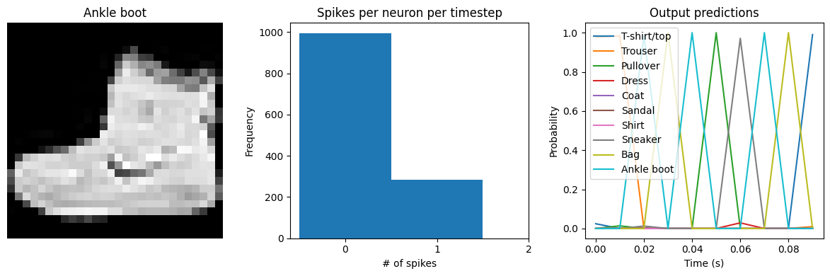
# plot output
for ii in range(4):
plt.figure(figsize=(12, 4))
plt.subplot(1, 3, 1)
plt.title(class_names[test_labels[ii]])
plt.imshow(test_images[ii], cmap="gray")
plt.axis("off")
plt.subplot(1, 3, 2)
plt.title("Spikes per neuron per timestep")
bin_edges = np.arange(int(np.max(n_spikes[ii])) + 2) - 0.5
plt.hist(np.ravel(n_spikes[ii]), bins=bin_edges)
x_ticks = plt.xticks()[0]
plt.xticks(
x_ticks[(np.abs(x_ticks - np.round(x_ticks)) < 1e-8) & (x_ticks > -1e-8)]
)
plt.xlabel("# of spikes")
plt.ylabel("Frequency")
plt.subplot(1, 3, 3)
plt.title("Output predictions")
plt.plot(
np.arange(test_sequences.shape[1]) * func_model.spike_layer.dt,
torch.softmax(torch.tensor(output[ii]), dim=-1),
)
plt.legend(class_names, loc="upper left")
plt.xlabel("Time (s)")
plt.ylabel("Probability")
plt.ylim([-0.05, 1.05])
plt.tight_layout()
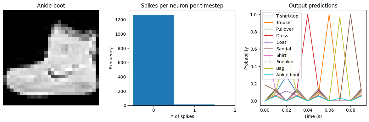
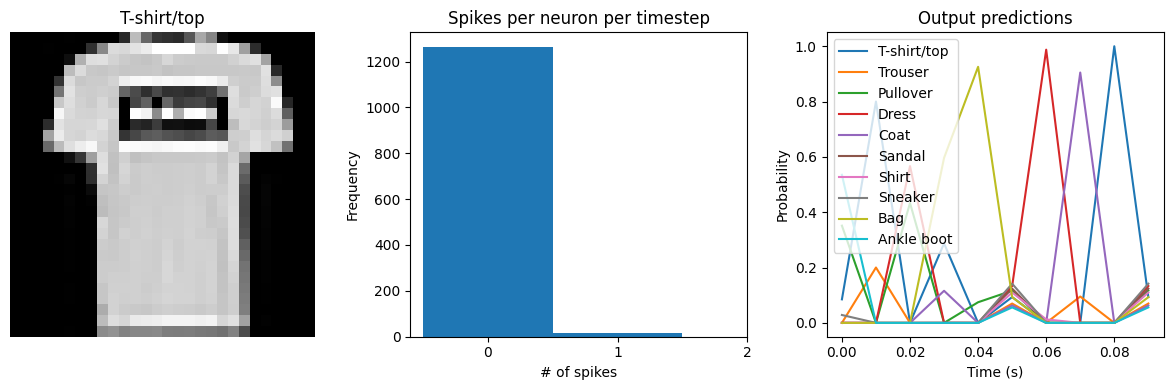
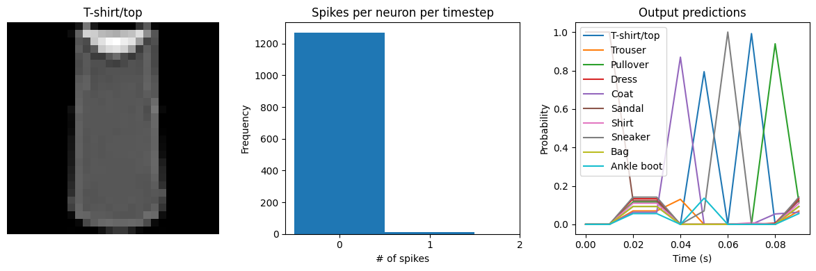
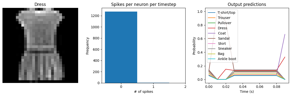
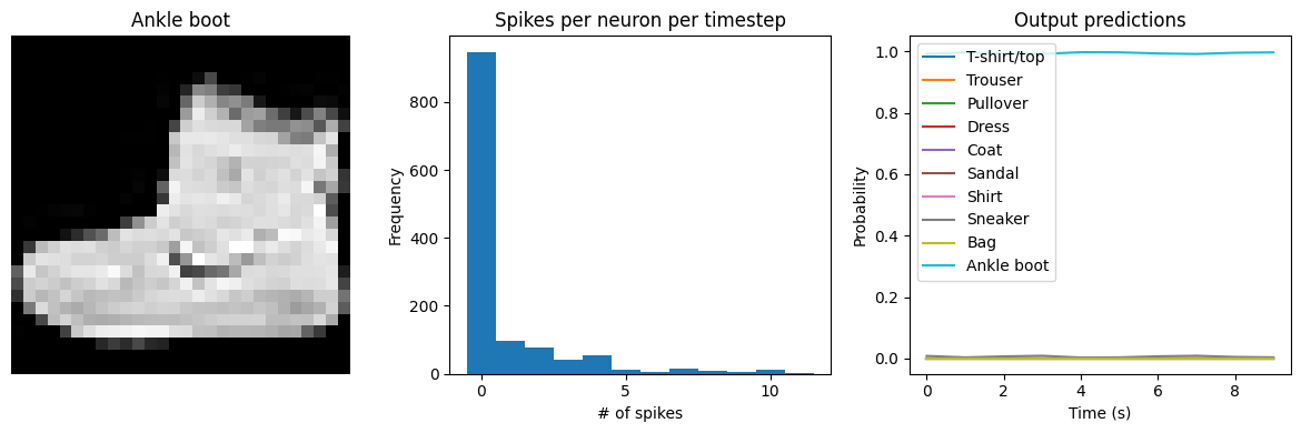
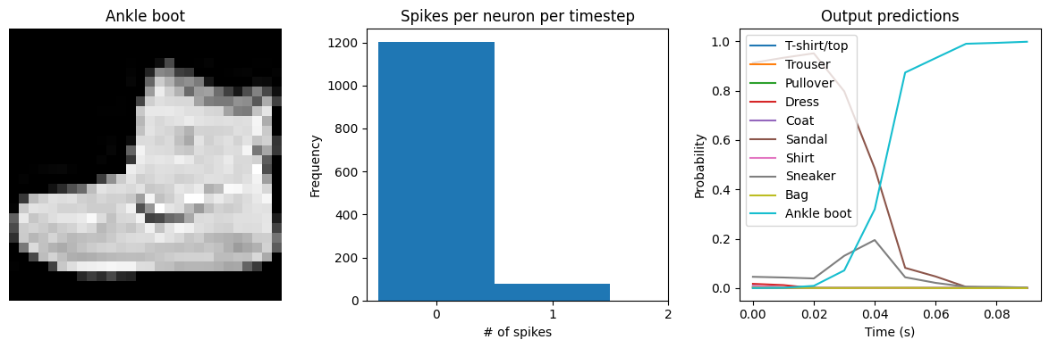
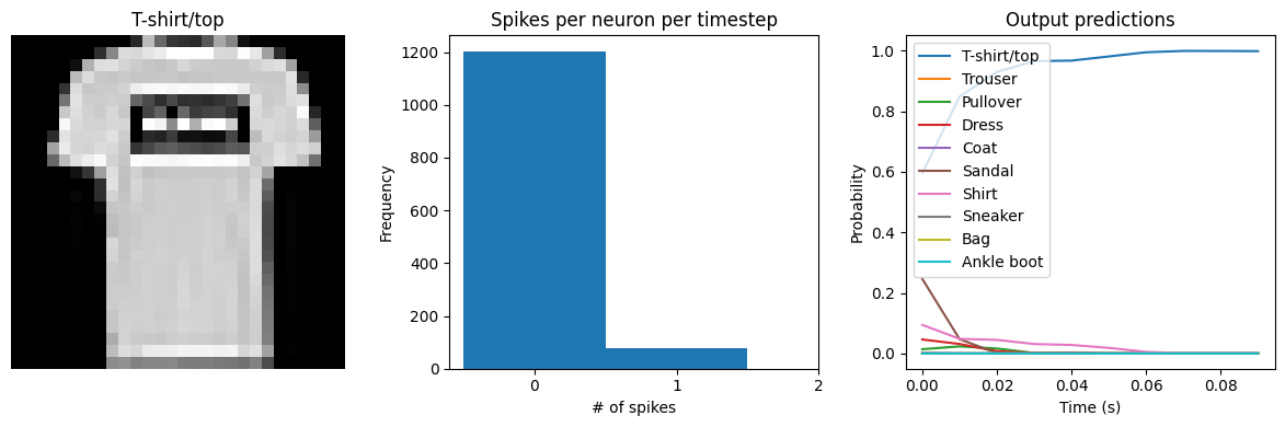
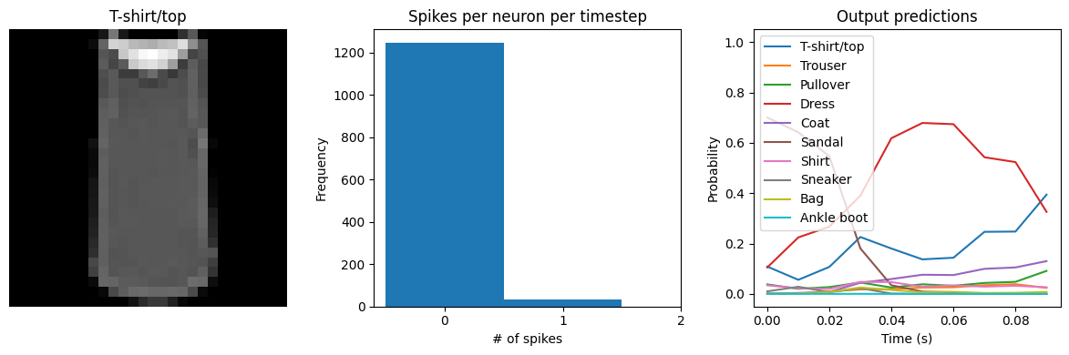
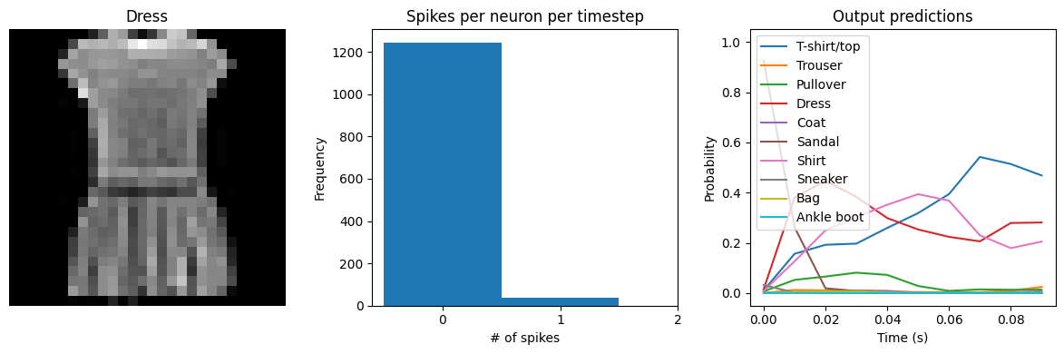
[7]:
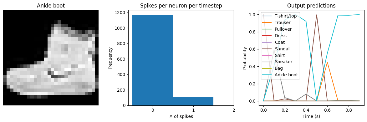
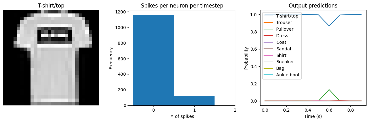
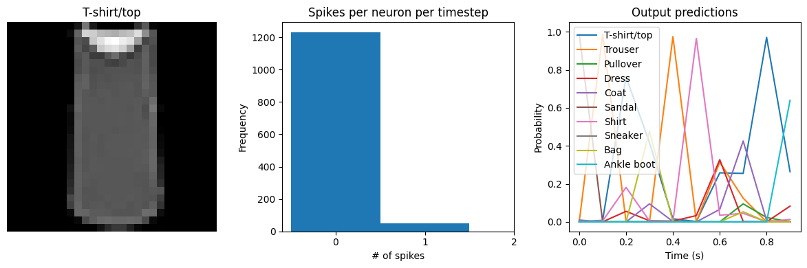
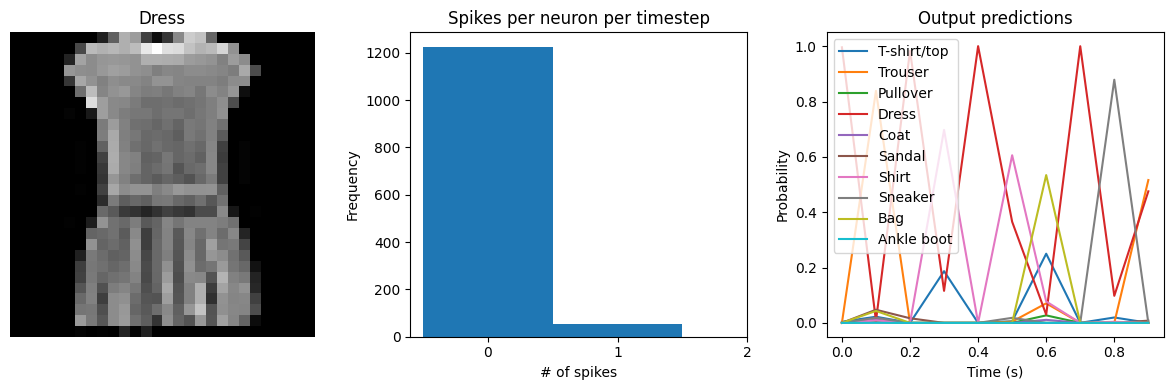
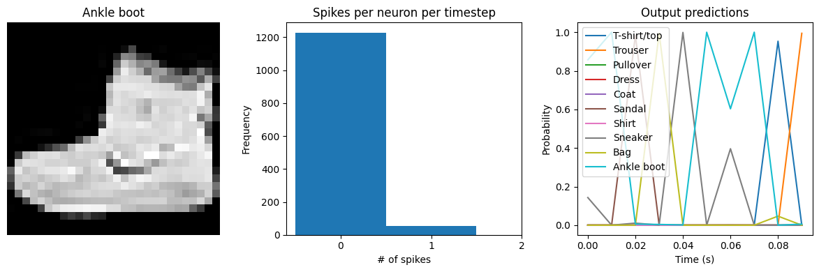
check_output(spiking_model)
Test accuracy: 17.85
Spike rate per neuron (Hz): min=0.00 mean=0.61 max=100.00
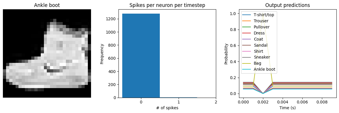
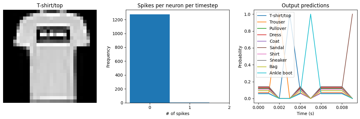
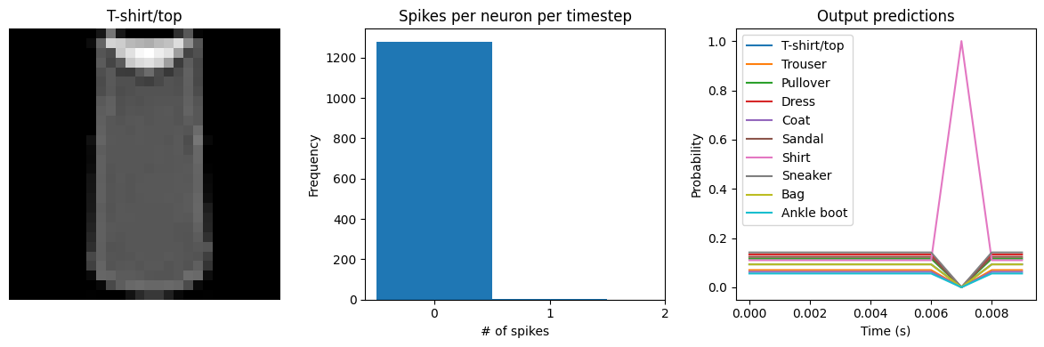
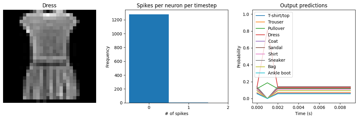
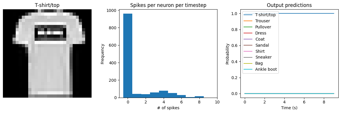
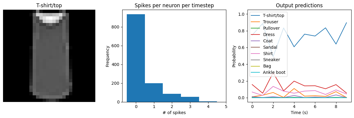
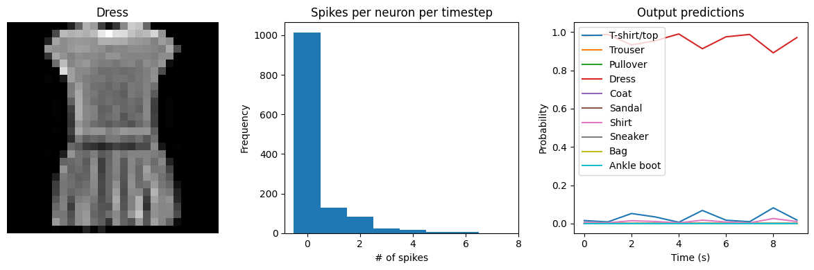
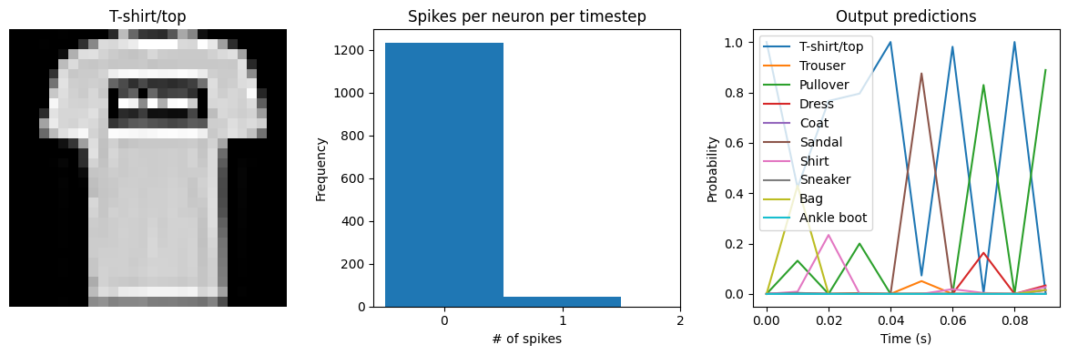
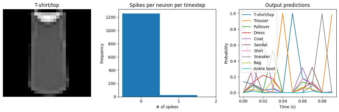
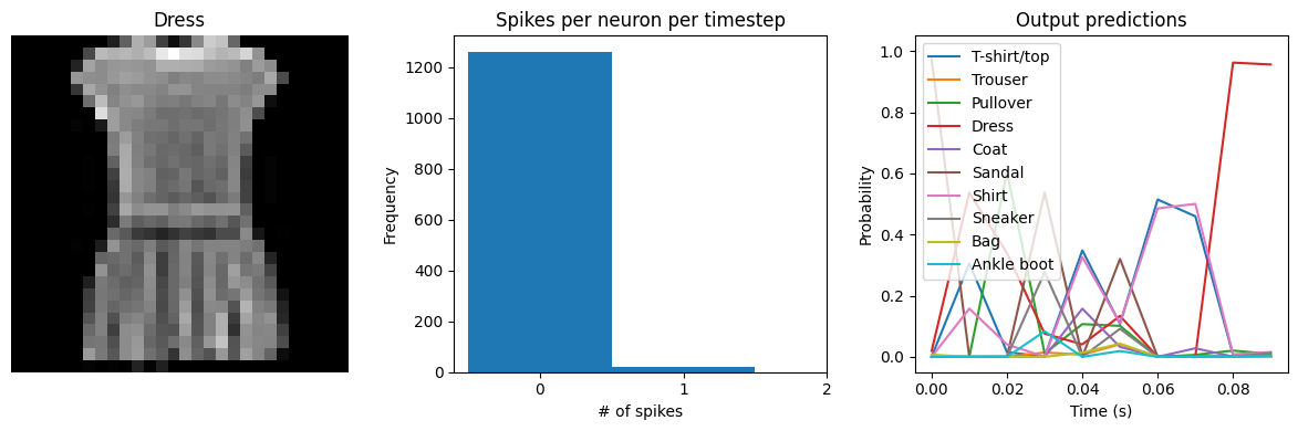
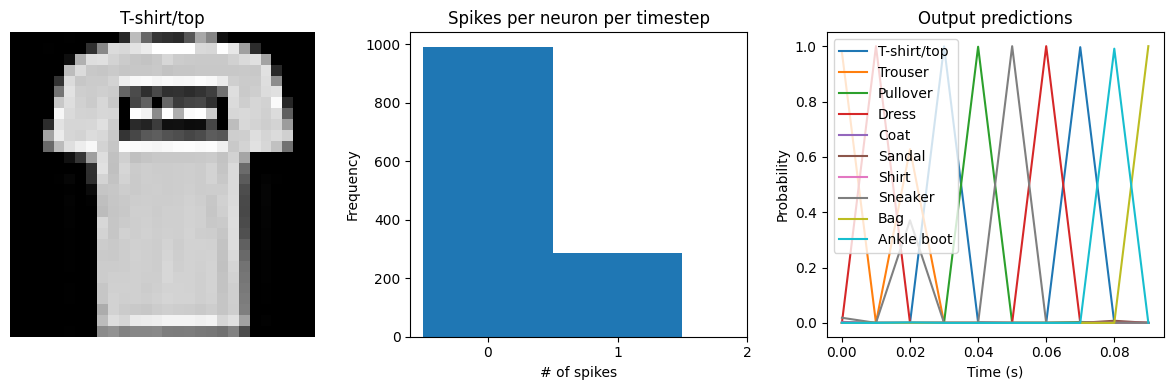
We can see an immediate problem: the neurons are hardly spiking at all. The mean number of spikes we’re getting out of each neuron in our SpikingActivation layer is very close to zero, and as a result the output is mostly flat.
To help understand why, we need to think more about the temporal nature of spiking neurons. Recall that the layer is set up such that if the base activation function were to be outputting a value of 1, the spiking equivalent would be spiking at 1Hz (i.e., emitting one spike per second). In the above example we are simulating for 10 timesteps, with the default dt of 0.001s, so we’re simulating a total of 0.01s. If our neurons aren’t spiking very rapidly, and we’re only simulating for 0.01s,
then it’s not surprising that we aren’t getting any spikes in that time window.
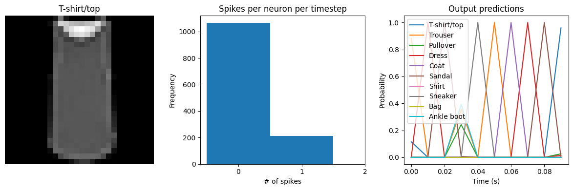
We can increase the value of dt, effectively running the spiking neurons for longer, in order to get a more accurate measure of the neuron’s output. Basically this allows us to collect more spikes from each neuron, giving us a better estimate of the neuron’s actual spike rate. We can see how the number of spikes and accuracy change as we increase dt:
[8]:
# dt=0.01 * 10 timesteps is equivalent to 0.1s of simulated time
check_output(spiking_model, modify_dt=0.01)
Test accuracy: 64.42
Spike rate per neuron (Hz): min=0.00 mean=0.60 max=30.00
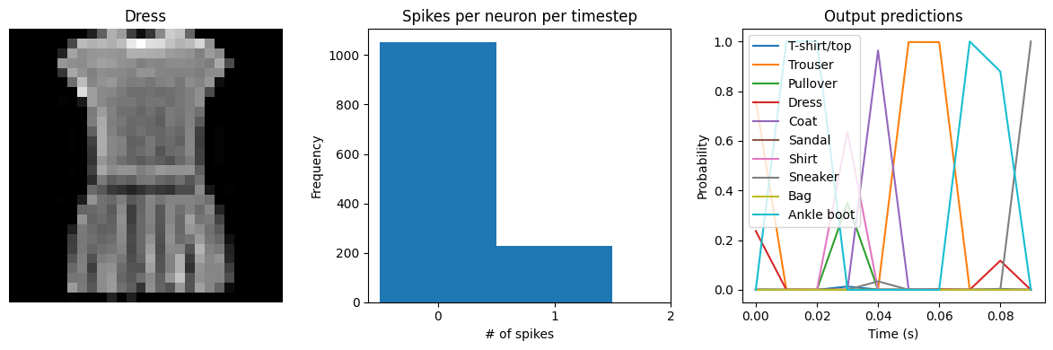
[9]:
check_output(spiking_model, modify_dt=0.1)
Test accuracy: 90.32
Spike rate per neuron (Hz): min=0.00 mean=0.61 max=24.00
[10]:
check_output(spiking_model, modify_dt=1)
Test accuracy: 90.68
Spike rate per neuron (Hz): min=0.00 mean=0.61 max=24.50
We can see that as we increase dt the performance of the spiking model increasingly approaches the non-spiking performance. In addition, as dt increases, the number of spikes is increasing. To understand why this improves accuracy, keep in mind that although the simulated time is increasing, the actual number of timesteps is still 10 in all cases. We’re effectively binning all the spikes that occur on each time step. So as our bin sizes get larger (increasing dt), the spike counts
will more closely approximate the “true” output of the underlying non-spiking activation function.
One might be tempted to simply increase dt to a very large value, and thereby always get great performance. But keep in mind that when we do that we have likely lost any of the advantages that were motivating us to investigate spiking models in the first place. For example, one prominent advantage of spiking models is temporal sparsity (we only need to communicate occasional spikes, rather than continuous values). However, with large dt the neurons are likely spiking every simulation
time step (or multiple times per timestep), so the activity is no longer temporally sparse.
Thus setting dt represents a trade-off between accuracy and temporal sparsity. Choosing the appropriate value will depend on the demands of your application.
Spiking aware training
As mentioned above, by default SpikingActivation layers will use the non-spiking activation function during training and the spiking version during inference. However, similar to the idea of quantization aware training, often we can improve performance by partially incorporating spiking behaviour during training. Specifically, we will use the spiking activation on the forward pass, while still using the non-spiking version on the backwards pass. This allows the model to learn weights that account for the discrete, temporal nature of the spiking activities.
[11]:
spikeaware_model = torch.nn.Sequential(
    torch.nn.Linear(784, 128),
    # set spiking_aware_training and a moderate dt
    pytorch_spiking.SpikingActivation(
        torch.nn.ReLU(), dt=0.01, spiking_aware_training=True
    ),
    pytorch_spiking.TemporalAvgPool(),
    torch.nn.Linear(128, 10),
)

train(spikeaware_model, train_sequences, test_sequences)
Train accuracy (0): 0.6973999738693237
Train accuracy (1): 0.7862666845321655
Train accuracy (2): 0.8085166811943054
Train accuracy (3): 0.8195000290870667
Train accuracy (4): 0.8271499872207642
Train accuracy (5): 0.8342499732971191
Train accuracy (6): 0.8389000296592712
Train accuracy (7): 0.84375
Train accuracy (8): 0.8477333188056946
Train accuracy (9): 0.8498499989509583
Test accuracy: 0.8520500063896179
[12]:
check_output(spikeaware_model)
Test accuracy: 85.33
Spike rate per neuron (Hz): min=0.00 mean=2.73 max=70.00
We can see that with spiking_aware_training we’re getting better performance than we were with the equivalent dt value above. The model has learned weights that are less sensitive to the discrete, sparse output produced by the spiking neurons.
Spike rate regularization
As we saw in the Simulation time section, the spiking rate of the neurons is very important. If a neuron is spiking too slowly then we don’t have enough information to determine its output value. Conversely, if a neuron is spiking too quickly then we may lose the spiking advantages we are looking for, such as temporal sparsity.
Thus it can be helpful to more directly control the firing rates in the model by applying regularization penalties during training. For example, we could add an L2 penalty to the output of the spiking activation layer.
[13]:
# construct model using a generic Module so that we can
# access the spiking activations in our loss function
class Model(torch.nn.Module):
    def __init__(self):
        super().__init__()

        self.dense0 = torch.nn.Linear(784, 128)
        self.spiking_activation = pytorch_spiking.SpikingActivation(
            torch.nn.ReLU(), dt=0.01, spiking_aware_training=True
        )
        self.temporal_pooling = pytorch_spiking.TemporalAvgPool()
        self.dense1 = torch.nn.Linear(128, 10)

    def forward(self, inputs):
        x = self.dense0(inputs)
        spikes = self.spiking_activation(x)
        spike_rates = self.temporal_pooling(spikes)
        output = self.dense1(spike_rates)

        return output, spike_rates


regularized_model = Model()

minibatch_size = 32
optimizer = torch.optim.Adam(regularized_model.parameters())

regularized_model.train()
for j in range(10):
    train_acc = 0
    for i in range(train_sequences.shape[0] // minibatch_size):
        regularized_model.zero_grad()

        batch_in = train_sequences[i * minibatch_size : (i + 1) * minibatch_size]
        batch_in = batch_in.reshape((-1,) + train_sequences.shape[1:-2] + (784,))
        batch_label = train_labels[i * minibatch_size : (i + 1) * minibatch_size]
        output, spike_rates = regularized_model(torch.tensor(batch_in))

        # compute sparse categorical cross entropy loss
        logp = torch.nn.functional.log_softmax(output, dim=-1)
        logpy = torch.gather(logp, 1, torch.tensor(batch_label).view(-1, 1))
        loss = -logpy.mean()

        # add activity regularization
        reg_weight = 1e-3  # weight on regularization penalty
        target_rate = 20  # target spike rate (in Hz)
        loss += reg_weight * torch.mean(
            torch.sum((spike_rates - target_rate) ** 2, dim=-1)
        )

        loss.backward()
        optimizer.step()

        train_acc += torch.mean(
            torch.eq(torch.argmax(output, dim=1), torch.tensor(batch_label)).float()
        )

    train_acc /= i + 1
    print(f"Train accuracy ({j}): {train_acc.numpy()}")
Train accuracy (0): 0.5892666578292847
Train accuracy (1): 0.6871833205223083
Train accuracy (2): 0.7019666433334351
Train accuracy (3): 0.7109833359718323
Train accuracy (4): 0.7110833525657654
Train accuracy (5): 0.7173833250999451
Train accuracy (6): 0.7180666923522949
Train accuracy (7): 0.7201333045959473
Train accuracy (8): 0.720633327960968
Train accuracy (9): 0.7221666574478149
[14]:
check_output(regularized_model)
Test accuracy: 71.15
Spike rate per neuron (Hz): min=0.00 mean=18.97 max=40.00
We can see that the spike rates have moved towards the 20 Hz target we specified. However, the test accuracy has dropped, since we’re adding an additional optimization constraint. (The accuracy is still higher than the original result with dt=0.01, due to the higher spike rates.) We could lower the regularization weight to allow more freedom in the firing rates. Again, this is a tradeoff that is made between controlling the firing rates and optimizing accuracy, and the best value for that
tradeoff will depend on the particular application (e.g., how important is it that spike rates fall within a particular range?).
Lowpass filtering
Another tool we can employ when working with SpikingActivation layers is filtering. As we’ve seen, the output of a spiking layer consists of discrete, temporally sparse spike events. This makes it difficult to determine the spike rate of a neuron when just looking at a single timestep. In the cases above we have worked around this by using a TemporalAveragePooling layer to average the output across all timesteps before classification.
Another way to achieve this is to compute some kind of moving average of the spiking output across timesteps. This is effectively what filtering is doing. PyTorchSpiking contains a Lowpass layer, which implements a lowpass filter. This has a parameter tau, known as the filter time constant, which controls the degree of smoothing the layer will apply. Larger tau values will apply more smoothing, meaning that we’re aggregating information
across longer periods of time, but the output will also be slower to adapt to changes in the input.
By default the tau values are trainable. We can use this in combination with spiking aware training to enable the model to learn time constants that best trade off spike noise versus response speed.
Unlike pytorch_spiking.TemporalAvgPool, pytorch_spiking.Lowpass computes outputs for all timesteps by default. This makes it possible to apply filtering throughout the model—not only on the final layer—in the case that there are multiple spiking layers. For the final layer, we can pass return_sequences=False to have the layer only return the output of the final timestep, rather than the outputs of all timesteps.
[15]:
dt = 0.01

filtered_model = torch.nn.Sequential(
    torch.nn.Linear(784, 128),
    pytorch_spiking.SpikingActivation(
        torch.nn.ReLU(), spiking_aware_training=True, dt=dt
    ),
    # add a lowpass filter on output of spiking layer
    # note: the lowpass dt doesn't necessarily need to be the same as the
    # SpikingActivation dt, but it's probably a good idea to keep them in sync
    # so that if we change dt the relative effect of the lowpass filter is unchanged
    pytorch_spiking.Lowpass(units=128, tau=0.1, dt=dt, return_sequences=False),
    torch.nn.Linear(128, 10),
)

train(filtered_model, train_sequences, test_sequences)
Train accuracy (0): 0.7164333462715149
Train accuracy (1): 0.7952166795730591
Train accuracy (2): 0.8166833519935608
Train accuracy (3): 0.8273166418075562
Train accuracy (4): 0.8357999920845032
Train accuracy (5): 0.8395833373069763
Train accuracy (6): 0.8468166589736938
Train accuracy (7): 0.8513666391372681
Train accuracy (8): 0.8546500205993652
Train accuracy (9): 0.8572666645050049
Test accuracy: 0.8612333536148071
[16]:
check_output(filtered_model)
Test accuracy: 86.21
Spike rate per neuron (Hz): min=0.00 mean=4.27 max=70.00
We can see that the model performs similarly to the previous spiking aware training example, which makes sense since, for a static input image, a moving average is very similar to a global average. We would need a more complicated model, with multiple spiking layers or inputs that are changing over time, to really see the benefits of a Lowpass layer.
Summary
We can use SpikingActivation layers to convert any activation function to an equivalent spiking implementation. Models with SpikingActivations can be trained and evaluated in the same way as non-spiking models, thanks to the swappable training/inference behaviour.
There are also a number of additional features that should be kept in mind in order to optimize the performance of a spiking model:
Simulation time: by adjusting
dtwe can trade off temporal sparsity versus accuracySpiking aware training: incorporating spiking dynamics on the forward pass can allow the model to learn weights that are more robust to spiking activations
Spike rate regularization: we can gain more control over spike rates by directly incorporating activity regularization into the optimization process
Lowpass filtering: we can achieve better accuracy with fewer spikes by aggregating spike data over time