
- Introduction
- Installation
- User guide
- API reference
- Examples
- Coming from Nengo to NengoDL
- Coming from TensorFlow to NengoDL
- Integrating a Keras model into a Nengo network
- Optimizing a spiking neural network
- Converting a Keras model to a spiking neural network
- Legendre Memory Units in NengoDL
- Optimizing a cognitive model
- Optimizing a cognitive model with temporal dynamics
- Additional resources
- Project information
Optimizing a cognitive model
![]()
The purpose of this example is to illustrate how NengoDL can be used to optimize a more complex cognitive model, involving the retrieval of information from highly structured semantic pointers. We will create a network that takes a collection of information as input (encoded using semantic pointers), and train it to retrieve some specific element from that collection.
[1]:
%matplotlib inline

from urllib.request import urlretrieve

import matplotlib.pyplot as plt
import nengo
from nengo import spa
import numpy as np
import tensorflow as tf

import nengo_dl
The first thing to do is define a function that produces random examples of structured semantic pointers. Each example consists of a collection of role-filler pairs of the following form:
\(TRACE_0 = \sum_{j=0}^N Role_{0,j} \circledast Filler_{0,j}\)
where terms like \(Role\) refer to simpler semantic pointers (i.e., random vectors), the \(\circledast\) symbol denotes circular convolution, and the summation means vector addition. That is, we define different pieces of information consisting of Roles and Fillers, and then we sum the information together in order to generate the full trace. As an example of how this might look in practice, we could encode information about a dog as
\(DOG = COLOUR \circledast BROWN + LEGS \circledast FOUR + TEXTURE \circledast FURRY + ...\)
The goal of the system is then to retrieve a cued piece of information from the semantic pointer. For example, if we gave the network the trace \(DOG\) and the cue \(COLOUR\) it should output \(BROWN\).
[2]:
def get_data(n_items, pairs_per_item, vec_d, vocab_seed):
    # the vocabulary object will handle the creation of semantic
    # pointers for us
    rng = np.random.RandomState(vocab_seed)
    vocab = spa.Vocabulary(dimensions=vec_d, rng=rng, max_similarity=1)

    # initialize arrays of shape (n_inputs, n_steps, vec_d)
    traces = np.zeros((n_items, 1, vec_d))
    cues = np.zeros((n_items, 1, vec_d))
    targets = np.zeros((n_items, 1, vec_d))

    # iterate through all of the examples to be generated
    for n in range(n_items):
        role_names = [f"ROLE_{n}_{i}" for i in range(pairs_per_item)]
        filler_names = [f"FILLER_{n}_{i}" for i in range(pairs_per_item)]

        # create key for the 'trace' of bound pairs (i.e. a
        # structured semantic pointer)
        trace_key = "TRACE_" + str(n)
        trace_ptr = vocab.parse(
            "+".join(f"{x} * {y}" for x, y in zip(role_names, filler_names))
        )
        trace_ptr.normalize()
        vocab.add(trace_key, trace_ptr)

        # pick which element will be cued for retrieval
        cue_idx = rng.randint(pairs_per_item)

        # fill array elements correspond to this example
        traces[n, 0, :] = vocab[trace_key].v
        cues[n, 0, :] = vocab[f"ROLE_{n}_{cue_idx}"].v
        targets[n, 0, :] = vocab[f"FILLER_{n}_{cue_idx}"].v

    return traces, cues, targets, vocab
Next we’ll define a Nengo model that retrieves cued items from structured semantic pointers. So, for a given trace (e.g., \(TRACE_0\)) and cue (e.g., \(Role_{0,0}\)), the correct output would be the corresponding filler (\(Filler_{0,0}\)). The model we’ll build will perform such retrieval by implementing a computation of the form:
\(TRACE_0 \:\: \circledast \sim Role_{0,0} \approx Filler_{0,0}\)
That is, convolving the trace with the inverse of the given cue will produce (approximately) the associated filler. More details about the mathematics of how/why this works can be found here.
We can create a model to perform this calculation by using the nengo.networks.CircularConvolution network that comes with Nengo.
[3]:
seed = 0
dims = 32
minibatch_size = 50
n_pairs = 2

with nengo.Network(seed=seed) as net:
    # use rectified linear neurons
    net.config[nengo.Ensemble].neuron_type = nengo.RectifiedLinear()
    net.config[nengo.Connection].synapse = None

    # provide a pointer and a cue as input to the network
    trace_inp = nengo.Node(np.zeros(dims))
    cue_inp = nengo.Node(np.zeros(dims))

    # create a convolution network to perform the computation
    # specified above
    cconv = nengo.networks.CircularConvolution(5, dims, invert_b=True)

    # connect the trace and cue inputs to the circular
    # convolution network
    nengo.Connection(trace_inp, cconv.input_a)
    nengo.Connection(cue_inp, cconv.input_b)

    # probe the output
    out = nengo.Probe(cconv.output)
In order to assess the retrieval accuracy of the model we need a metric for success. In this case we’ll say that a cue has been successfully retrieved if the output vector is more similar to the correct filler vector than it is to any of the other vectors in the vocabulary.
[4]:
def accuracy(output, vocab, targets, t_step=-1):
    # provide the probed output data, the vocab,
    # the target vectors, and the time step at which to evaluate

    # get output at the given time step
    output = output[:, t_step, :]

    # compute similarity between each output and vocab item
    sims = np.dot(vocab.vectors, output.T)
    idxs = np.argmax(sims, axis=0)

    # check that the output is most similar to the target
    acc = np.mean(np.all(vocab.vectors[idxs] == targets[:, 0], axis=1))

    return acc
Now we can run the model on some test data to check the baseline retrieval accuracy. Since we used only a small number of neurons in the circular convolution network, we should expect mediocre results.
[5]:
# generate some test inputs
test_traces, test_cues, test_targets, test_vocab = get_data(
    minibatch_size, n_pairs, dims, vocab_seed=seed
)
test_inputs = {trace_inp: test_traces, cue_inp: test_cues}

# run the simulator for one time step to compute the network outputs
with nengo_dl.Simulator(net, minibatch_size=minibatch_size) as sim:
    sim.step(data=test_inputs)

print("Retrieval accuracy:", accuracy(sim.data[out], test_vocab, test_targets))
Build finished in 0:00:01
Optimization finished in 0:00:00
Construction finished in 0:00:05
Retrieval accuracy: 0.06
These results indicate that the model is only rarely performing accurate retrieval, which means that this network is not very capable of manipulating structured semantic pointers in a useful way.
We can visualize the similarity of the output for one of the traces to get a sense of what this accuracy looks like (the similarity to the correct output is shown in red).
[6]:
plt.figure(figsize=(10, 5))
bars = plt.bar(
    np.arange(len(test_vocab.vectors)), np.dot(test_vocab.vectors, sim.data[out][0, 0])
)
bars[
    np.where(np.all(test_vocab.vectors == test_targets[0, 0], axis=1))[0][0]
].set_color("r")
plt.ylim([-1, 1])
plt.xlabel("Vocabulary items")
plt.ylabel("Similarity")
plt.show()
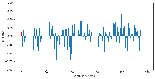
We can see that the actual output is not particularly similar to this desired output, which illustrates that the model is not performing accurate retrieval.
Now we’ll train the network parameters to improve performance. We won’t directly optimize retrieval accuracy, but will instead minimize the mean squared error between the model’s output vectors and the vectors corresponding to the correct output items for each input cue. We’ll use a large number of training examples that are distinct from our test data, so as to avoid explicitly fitting the model parameters to the test items.
To make this example run a bit quicker we’ll download some pretrained model parameters by default. Set do_training=True to train the model yourself.
[7]:
sim = nengo_dl.Simulator(net, minibatch_size=minibatch_size, seed=seed)

do_training = False
if do_training:
    # create training data and data feeds
    train_traces, train_cues, train_targets, _ = get_data(
        n_items=5000, pairs_per_item=n_pairs, vec_d=dims, vocab_seed=seed + 1
    )

    # train the model
    sim.compile(optimizer=tf.optimizers.RMSprop(2e-3), loss=tf.losses.mse)
    sim.fit(
        {trace_inp: train_traces, cue_inp: train_cues}, {out: train_targets}, epochs=100
    )

    sim.save_params("./spa_retrieval_params")

else:
    # download pretrained parameters
    urlretrieve(
        "https://drive.google.com/uc?export=download&"
        "id=1KmroagQpaDAVbN-VnozqWVJw_1xjKxZj",
        "spa_retrieval_params.npz",
    )

    # load parameters
    sim.load_params("./spa_retrieval_params")
Build finished in 0:00:01
Optimization finished in 0:00:00
Construction finished in 0:00:00
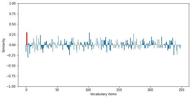
We can now recompute the network outputs using the trained model on the test data. We can see that the retrieval accuracy is significantly improved. You can modify the dimensionality of the vectors and the number of bound pairs in each trace to explore how these variables influence the upper bound on retrieval accuracy.
[8]:
sim.step(data=test_inputs)
print("Retrieval accuracy:", accuracy(sim.data[out], test_vocab, test_targets))
sim.close()
Retrieval accuracy: 0.86
[9]:
plt.figure(figsize=(10, 5))
bars = plt.bar(
    np.arange(len(test_vocab.vectors)), np.dot(test_vocab.vectors, sim.data[out][0, 0])
)
bars[
    np.where(np.all(test_vocab.vectors == test_targets[0, 0], axis=1))[0][0]
].set_color("r")
plt.ylim([-1, 1])
plt.xlabel("Vocabulary items")
plt.ylabel("Similarity")
plt.show()
Check out this example for a more complicated version of this task/model, in which a structured semantic pointer is built up over time by binding together sequentially presented input items.