- Overview
- Installation
- Configuration
- Example models
- API reference
- Tips and tricks
- Hardware setup
Nonlinear adaptive control
In this example, we will use the PES learning rule to learn the effects of gravity, applied to a 2-joint arm.
This example requires the abr_control library. To install it,
git clone https://github.com/abr/abr_control.git
pip install -e abr_control
Note that while this example uses a simualted 2-joint arm, the underlying network structure is identical to the network previously used to control a physical robot arm.
[1]:
%matplotlib inline
from abr_control.arms import twojoint as arm
from abr_control.controllers import OSC
import matplotlib.pyplot as plt
import nengo
import numpy as np

import nengo_loihi

nengo_loihi.set_defaults()
/home/travis/build/nengo/nengo-loihi/nengo_loihi/version.py:23: UserWarning: This version of `nengo_loihi` has not been tested with your `nengo` version (3.0.1.dev0). The latest fully supported version is 3.0.0
  "supported version is %s" % (nengo.__version__, latest_nengo_version)
/home/travis/virtualenv/python3.6.3/lib/python3.6/site-packages/nengo_dl/version.py:42: UserWarning: This version of `nengo_dl` has not been tested with your `nengo` version (3.0.1.dev0). The latest fully supported version is 3.0.0.
  % ((nengo.version.version,) + latest_nengo_version)
Creating the arm simulation and reaching framework
The first thing to do is create the arm simulation to simulate the dynamics of a two link arm, and an operational space controller to calculate what torques to apply to the joints to move the hand in a straight line to the targets.
[2]:
# set the initial position of the arm
robot_config = arm.Config(use_cython=True)
arm_sim = arm.ArmSim(
    robot_config=robot_config, dt=1e-3, q_init=[.95, 2.0])

# create an operational space controller
ctrlr = OSC(robot_config, kp=10, kv=7, vmax=[10, 10])
Robot has fewer DOF (2) than the specified number of space dimensions to control (3). Poor performance may result.
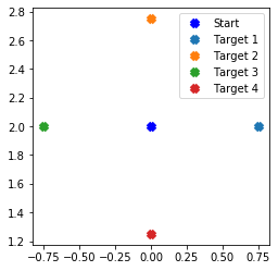
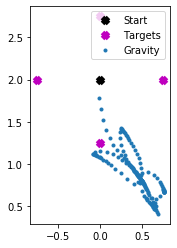
Next we create a set of targets for the arm to reach to. In this task the hand will start at a center location, then reach out and back to 4 targets around a circle.
[3]:
# create a set of targets to reach to
n_reaches = 4
distance = .75
center = [0, 2.0]
end_points = [[distance * np.cos(theta) + center[0],
               distance * np.sin(theta) + center[1]]
              for theta in np.linspace(0, 2*np.pi, n_reaches+1)][:-1]
targets = np.vstack([[center, ep] for ep in end_points])

plt.plot(center[0], center[1], 'bx', mew=5, label='Start')
for i, end_point in enumerate(end_points):
    plt.plot(end_point[0],
             end_point[1],
             'x',
             mew=5,
             label='Target %d' % (i + 1))
plt.gca().set_aspect('equal')
plt.legend()
[3]:
<matplotlib.legend.Legend at 0x7f57f28c8eb8>
[4]:
def build_baseline_model():
    with nengo.Network(label="Nonlinear adaptive control") as model:

        # Create node that specifies target
        def gen_target(t):
            # Advance to the next target in the list every 2 seconds
            return targets[int(t / 2) % len(targets)]
        target_node = nengo.Node(output=gen_target, size_out=2)

        # Create node that calculates the OSC signal
        model.osc_node = nengo.Node(
            output=lambda t, x: ctrlr.generate(
                q=x[:2], dq=x[2:4], target=np.hstack([x[4:6], np.zeros(4)])),
            size_in=6, size_out=2)

        # Create node that runs the arm simulation and gets feedback
        def arm_func(t, x):
            u = x[:2]  # the OSC signal
            u += x[2:4] * 10  # add in the adaptive control signal
            arm_sim.send_forces(u)  # step the arm simulation forward
            # return arm joint angles, joint velocities, and hand (x,y)
            return np.hstack([arm_sim.q, arm_sim.dq, arm_sim.x])
        model.arm_node = nengo.Node(output=arm_func, size_in=4)

        # hook up the OSC controller and arm simulation
        nengo.Connection(model.osc_node, model.arm_node[:2])
        nengo.Connection(model.arm_node[:4], model.osc_node[:4])
        # send in current target to the controller
        nengo.Connection(target_node, model.osc_node[4:6])

        model.probe_target = nengo.Probe(target_node)  # track targets
        model.probe_hand = nengo.Probe(model.arm_node[4:6])  # track hand (x,y)
        model.probe_q = nengo.Probe(model.arm_node[:2])  # track joint angles

    return model


baseline_model = build_baseline_model()
Generating transform function for joint0[0,0,0]_Tx
Generating transform function for joint1[0,0,0]_Tx
Generating transform function for EE[0,0,0]_Tx
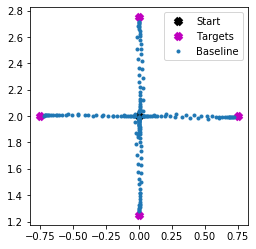
Running the network in Nengo
We can now run the basic framework, where the operational space controller will drive the hand to the 4 targets around the circle.
[5]:
# each reach is 2 seconds out + 2 seconds back in
runtime = n_reaches * 2 * 2 + 2

arm_sim.reset()
with nengo.Simulator(baseline_model, progress_bar=False) as sim:
    sim.run(runtime)
baseline_t = sim.trange()
baseline_data = sim.data
Generating Jacobian function for EE[0,0,0]_J
Loading expression from EE[0,0,0]_Tx ...
Generating inertia matrix function
Generating Jacobian function for link0[0,0,0]_J
Generating transform function for link0[0,0,0]_Tx
Generating Jacobian function for link1[0,0,0]_J
Generating transform function for link1[0,0,0]_Tx
Generating Jacobian function for link2[0,0,0]_J
Generating transform function for link2[0,0,0]_Tx
Generating Jacobian function for joint0[0,0,0]_J
Loading expression from joint0[0,0,0]_Tx ...
Generating Jacobian function for joint1[0,0,0]_J
Loading expression from joint1[0,0,0]_Tx ...
Generating gravity compensation function
Loading expression from link0[0,0,0]_J ...
Loading expression from link1[0,0,0]_J ...
Loading expression from link2[0,0,0]_J ...
Loading expression from joint0[0,0,0]_J ...
Loading expression from joint1[0,0,0]_J ...
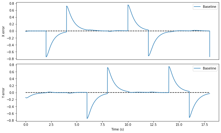
The error is calculated as the difference between the hand (x,y) position and the target. Whenever the target changes, the error will jump up, and then quickly decrease as the hand approaches the target.
[6]:
def calculate_error(model, data):
    return data[model.probe_hand] - data[model.probe_target]


baseline_error = calculate_error(baseline_model, baseline_data)


def plot_data(t_set, data_set, label_set):
    plt.figure(figsize=(10, 6))
    plt.title("Distance to target")

    ax1 = plt.subplot(2, 1, 1)
    ax1.plot(t_set[0], np.zeros_like(t_set[0]), 'k--')
    plt.xticks([])
    plt.ylabel('X error')

    ax2 = plt.subplot(2, 1, 2)
    ax2.plot(t_set[0], np.zeros_like(t_set[0]), 'k--')
    plt.ylabel('Y error')
    plt.xlabel("Time (s)")

    plt.tight_layout()

    for t, data, label in zip(t_set, data_set, label_set):
        ax1.plot(t, data[:, 0], label=label)
        ax2.plot(t, data[:, 1], label=label)

    ax1.legend(loc=1)
    ax2.legend(loc=1)


def plot_xy(t_set, data_set, label_set):
    tspace = 0.1
    ttol = 1e-5

    plt.figure()
    ax = plt.subplot(111)
    ax.plot(center[0], center[1], 'kx', mew=5, label='Start')
    ax.plot([p[0] for p in end_points], [p[1] for p in end_points],
            'mx', mew=5, label='Targets')
    for t, data, label in zip(t_set, data_set, label_set):
        tmask = (t + ttol) % tspace < 2*ttol
        ax.plot(data[tmask, 0], data[tmask, 1], '.', label=label)
    ax.legend(loc=1)
    ax.set_aspect('equal')


plot_xy(
    [baseline_t],
    [baseline_data[baseline_model.probe_hand]],
    ['Baseline'])
plot_data(
    [baseline_t],
    [baseline_error],
    ['Baseline'])
Adding unexpected gravity
Now we add gravity along the y-axis to the 2-link arm model, which it is not expecting. As a result, the error will be much greater as it tries to reach to the various targets relative to baseline performance. Note that although gravity is only applied along the y-axis, because the arm joints are not all oriented vertically, the effect of gravity on the arm segments also pulls the hand along the x-axis.
[7]:
def add_gravity(model):
    with model:
        # calculate and add in gravity along y axis
        gravity = np.array([0, -9.8, 0, 0, 0, 0])
        M0g = np.dot(robot_config._M_LINKS[0], gravity)
        M1g = np.dot(robot_config._M_LINKS[1], gravity)

        def gravity_func(t, q):
            g = np.dot(robot_config.J('link1', q=q).T, M0g)
            g += np.dot(robot_config.J('link2', q=q).T, M1g)
            return g
        gravity_node = nengo.Node(gravity_func, size_in=2, size_out=2)
        # connect perturbation to arm
        nengo.Connection(model.arm_node[:2], gravity_node)
        nengo.Connection(gravity_node, model.arm_node[:2])

    return model


gravity_model = add_gravity(build_baseline_model())
[8]:
arm_sim.reset()
with nengo.Simulator(gravity_model, progress_bar=False) as sim:
    sim.run(runtime)
gravity_t = sim.trange()
gravity_data = sim.data
Loading expression from link1[0,0,0]_J ...
Loading expression from link2[0,0,0]_J ...
[9]:
gravity_error = calculate_error(gravity_model, gravity_data)
plot_xy(
    [gravity_t],
    [gravity_data[gravity_model.probe_hand]],
    ['Gravity'])
plot_data(
    [baseline_t, gravity_t],
    [baseline_error, gravity_error],
    ['Baseline', 'Gravity'])
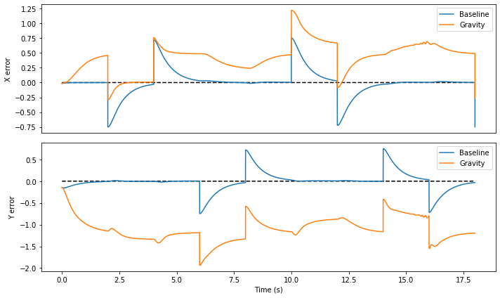
As expected, the error is much worse, especially along the Y axis (take note of the scale of the axes), because gravity is affecting the system and the operational space controller is not accounting for it.
Adding nonlinear adaptive control
Now we add in an ensemble of neurons to perform context sensitive error integration, as presented in DeWolf, Stewart, Slotine, and Eliasmith, 2015. We want the context for adaptation to be the joint angles of the arm. For optimal performance, the input to the ensemble should be in the range -1 to 1, so we need to look at the expected range of joint angles and transform the input signal accordingly.
[10]:
for ii in range(2):
    plt.subplot(2, 1, ii+1)
    plt.plot(sim.trange(),
             baseline_data[baseline_model.probe_q][:, ii],
             label='Baseline')
    plt.plot(sim.trange(),
             gravity_data[gravity_model.probe_q][:, ii],
             label='Gravity')
    plt.ylabel('Joint %i' % ii)
    plt.legend()
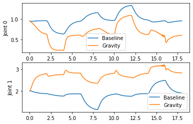
Looking at this data, we can estimate the mean of Joint 0 across the two runs to be around .75, with a range of .75 to either side of the mean. For Joint 1 it’s a bit more difficult; we’re going to err to the Baseline values with the hope the adaptive controller helps keep us in that range. So we’ll choose a mean of 2 and range of 1 to either side of the mean.
[11]:
def add_adaptation(model, learning_rate=1e-5):
    with model:
        # create ensemble to adapt to unmodeled dynamics
        adapt = nengo.Ensemble(n_neurons=1000, dimensions=2, radius=np.sqrt(2))

        means = np.array([.75, 2.25])
        scaling = np.array([.75, 1.25])
        scale_node = nengo.Node(
            output=lambda t, x: (x - means) / scaling,
            size_in=2,
            size_out=2)
        # to send target info to ensemble
        nengo.Connection(model.arm_node[:2], scale_node)
        nengo.Connection(scale_node, adapt)

        # create the learning connection from adapt to the arm simulation
        learn_conn = nengo.Connection(
            adapt, model.arm_node[2:4],
            function=lambda x: np.zeros(2),
            learning_rule_type=nengo.PES(learning_rate),
            synapse=0.05)
        # connect up the osc signal as the training signal
        nengo.Connection(
            model.osc_node, learn_conn.learning_rule, transform=-1)
    return model


adapt_model = add_adaptation(add_gravity(build_baseline_model()))
[12]:
arm_sim.reset()
with nengo.Simulator(adapt_model, progress_bar=False) as sim:
    sim.run(runtime)
adapt_t = sim.trange()
adapt_data = sim.data
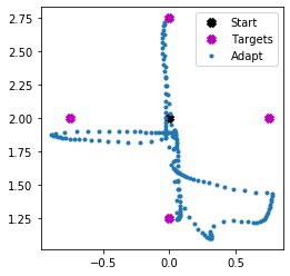
[13]:
adapt_error = calculate_error(adapt_model, adapt_data)
plot_xy(
    [adapt_t],
    [adapt_data[adapt_model.probe_hand]],
    ['Adapt'])
plot_data(
    [baseline_t, gravity_t, adapt_t],
    [baseline_error, gravity_error, adapt_error],
    ['Baseline', 'Gravity', 'Gravity + Adapt'])
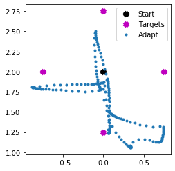
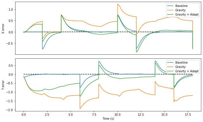
And we can see that even in only one pass through the target set the adaptive ensemble has already significantly reduced the error. To see further reductions, change the run time of the simulation to be longer so that the arm does multiple passes of the target set (by changing sim.run(runtime) to sim.run(runtime*2)).
Running the network with Nengo Loihi
Loihi has limits on the magnitude of the error signal, so we need to adjust the pes_error_scale parameter to avoid too much overflow.
[14]:
arm_sim.reset()

model = nengo_loihi.builder.Model()
model.pes_error_scale = 10

with nengo_loihi.Simulator(adapt_model, model=model) as sim:
    sim.run(runtime)
adapt_loihi_t = sim.trange()
adapt_loihi_data = sim.data
/home/travis/build/nengo/nengo-loihi/nengo_loihi/discretize.py:183: UserWarning: Received PES error greater than chip max (1.27e+01). Consider changing `Model.pes_error_scale`.
  "Consider changing `Model.pes_error_scale`." % (max_err / scale,)
/home/travis/build/nengo/nengo-loihi/nengo_loihi/discretize.py:193: UserWarning: Received PES error less than chip min (-1.27e+01). Consider changing `Model.pes_error_scale`.
  "Consider changing `Model.pes_error_scale`." % (-max_err / scale,)
[15]:
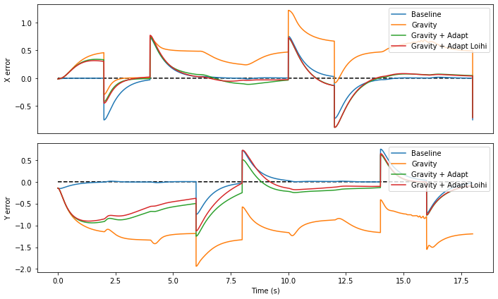
adapt_loihi_error = calculate_error(adapt_model, adapt_loihi_data)
plot_xy(
    [adapt_loihi_t],
    [adapt_loihi_data[adapt_model.probe_hand]],
    ['Adapt'])
plot_data(
    [baseline_t, gravity_t, adapt_t, adapt_loihi_t],
    [baseline_error, gravity_error, adapt_error, adapt_loihi_error],
    ['Baseline', 'Gravity', 'Gravity + Adapt', 'Gravity + Adapt Loihi'])