CIFAR-10 convolutional network

This is a small CIFAR-10 convolutional neural network designed to run on one Loihi chip. Because of these size constraints, it is not particularly powerful, and does not achieve anywhere near state-of-the-art results on the task. Nevertheless, the network performs well enough to demonstrate that Loihi is capable of hosting larger, more powerful object recognition networks than MNIST.

The main libraries we’ll be using in this tutorial are:

• nengo to create the network

• nengo_dl to train the network (nengo_dl uses tensorflow under the hood, so we also import that, along with the tensorflow_probability extension package, to define the loss function)

• nengo_loihi to run the network on the Loihi hardware (or simulate Loihi if hardware is not available)

%matplotlib inline

import collections
from functools import partial
from urllib.request import urlretrieve

import matplotlib.pyplot as plt
import nengo
import nengo_dl
import numpy as np
import tensorflow as tf
import tensorflow_probability as tfp

import nengo_loihi

Preliminaries

First, we’ll make some preliminary definitions that will help us throughout the rest of the training process. Understanding these in detail is not necessary to understand the example, so feel free to skip them and come back later, or ignore them completely.

We define a function called percentile_l2_loss_range, which we will use to help regularize our neuron firing rates so that they fall in our desired range. The input y to our function is the firing rates of all neurons across all examples in the batch. We compute a percentile on these firing rates for each neuron, across all the examples. If this percentile is outside our desired range of min to max, then it contributes to the squared loss.

slice_data_dict applies a slice to the first dimension of all arrays in a data dictionary, to make it easy to select a subset of data for testing.

def percentile_l2_loss_range(
    y_true, y, sample_weight=None, min_rate=0.0, max_rate=np.inf, percentile=99.0
):
    # y axes are (batch examples, time (==1), neurons)
    assert len(y.shape) == 3
    rates = tfp.stats.percentile(y, percentile, axis=(0, 1))
    low_error = tf.maximum(0.0, min_rate - rates)
    high_error = tf.maximum(0.0, rates - max_rate)
    loss = tf.nn.l2_loss(low_error + high_error)

    return (sample_weight * loss) if sample_weight is not None else loss


def slice_data_dict(data, slice_):
    return {key: value[slice_] for key, value in data.items()}

We also define a custom class for iterating an image dataset and returning dictionaries that can be used by NengoDL for training. Much of this is a re-implementation of tf.keras.preprocessing.image.NumpyArrayIterator, with the additional features of (a) allowing us to return dictionaries with the provided keys, rather than just lists of Numpy arrays, and (b) allowing multiple y values to be returned.

class NengoImageIterator(tf.keras.preprocessing.image.Iterator):
    def __init__(
        self,
        image_data_generator,
        x_keys,
        x,
        y_keys,
        y,
        batch_size=32,
        shuffle=False,
        sample_weight=None,
        seed=None,
        subset=None,
        dtype="float32",
    ):
        assert subset is None, "Not Implemented"
        assert isinstance(x_keys, (tuple, list))
        assert isinstance(y_keys, (tuple, list))
        assert isinstance(x, (tuple, list))
        assert isinstance(y, (tuple, list))

        self.dtype = dtype
        self.x_keys = x_keys
        self.y_keys = y_keys

        x0 = x[0]
        assert all(len(xx) == len(x0) for xx in x), (
            "All of the arrays in `x` should have the same length. "
            "[len(xx) for xx in x] = %s" % ([len(xx) for xx in x],)
        )
        assert all(len(yy) == len(x0) for yy in y), (
            "All of the arrays in `y` should have the same length as `x`. "
            "len(x[0]) = %d, [len(yy) for yy in y] = %s"
            % (len(x0), [len(yy) for yy in y])
        )
        assert len(x_keys) == len(x)
        assert len(y_keys) == len(y)

        if sample_weight is not None and len(x0) != len(sample_weight):
            raise ValueError(
                "`x[0]` (images tensor) and `sample_weight` "
                "should have the same length. "
                "Found: x.shape = %s, sample_weight.shape = %s"
                % (np.asarray(x0).shape, np.asarray(sample_weight).shape)
            )

        self.x = [
            np.asarray(xx, dtype=self.dtype if i == 0 else None)
            for i, xx in enumerate(x)
        ]
        if self.x[0].ndim != 4:
            raise ValueError(
                "Input data in `NumpyArrayIterator` "
                "should have rank 4. You passed an array "
                "with shape",
                self.x[0].shape,
            )

        self.y = [np.asarray(yy) for yy in y]
        self.sample_weight = (
            None if sample_weight is None else np.asarray(sample_weight)
        )
        self.image_data_generator = image_data_generator
        super().__init__(self.x[0].shape[0], batch_size, shuffle, seed)

    def _get_batches_of_transformed_samples(self, index_array):
        images = self.x[0]
        assert images.dtype == self.dtype

        n = len(index_array)
        batch_x = np.zeros((n,) + images[0].shape, dtype=self.dtype)
        for i, j in enumerate(index_array):
            x = images[j]
            params = self.image_data_generator.get_random_transform(x.shape)
            x = self.image_data_generator.apply_transform(x, params)
            x = self.image_data_generator.standardize(x)
            batch_x[i] = x

        batch_x_miscs = [xx[index_array] for xx in self.x[1:]]
        batch_y_miscs = [yy[index_array] for yy in self.y]

        x_pairs = [
            (k, self.x_postprocess(k, v))
            for k, v in zip(self.x_keys, [batch_x] + batch_x_miscs)
        ]
        y_pairs = [
            (k, self.y_postprocess(k, v)) for k, v in zip(self.y_keys, batch_y_miscs)
        ]

        output = (
            collections.OrderedDict(x_pairs),
            collections.OrderedDict(y_pairs),
        )

        if self.sample_weight is not None:
            output += (self.sample_weight[index_array],)
        return output

    def x_postprocess(self, key, x):
        return x if key == "n_steps" else x.reshape((x.shape[0], 1, -1))

    def y_postprocess(self, key, y):
        return y.reshape((y.shape[0], 1, -1))

Load the dataset

We load the CIFAR-10 dataset using TensorFlow. The data comes as numpy.uint8 values in the range [0, 255], so we rescale the data to the range [-1, 1]. We create one-hot representations of the labels to use during training, as well as “flat” versions of the data where the images are flattened into vectors. Finally, we define an input_shape object that describes the image shape in a format that Nengo can use.

One variable that occurs a number of times here is the channels_last option, which can be set to True or False. This option dictates whether the image (color) channels are stored as the last (i.e. least-significant) index in each image (True), or the first (i.e. most-significant) index (False). This will also dictate how the images will be represented on Loihi, and can have effects on the number of axons and weights required on the chip.

channels_last = True

(train_x, train_y), (test_x, test_y) = tf.keras.datasets.cifar10.load_data()

n_classes = len(np.unique(train_y))

# TensorFlow does not include the label names, so define them manually
label_names = [
    "airplane",
    "automobile",
    "bird",
    "cat",
    "deer",
    "dog",
    "frog",
    "horse",
    "ship",
    "truck",
]
assert n_classes == len(label_names)

if not channels_last:
    train_x = np.transpose(train_x, (0, 3, 1, 2))
    test_x = np.transpose(test_x, (0, 3, 1, 2))

# convert the images to float32, and rescale to [-1, 1]
train_x = train_x.astype(np.float32) / 127.5 - 1
test_x = test_x.astype(np.float32) / 127.5 - 1

train_t = np.array(tf.one_hot(train_y, n_classes), dtype=np.float32)
test_t = np.array(tf.one_hot(test_y, n_classes), dtype=np.float32)

train_y = train_y.squeeze()
test_y = test_y.squeeze()

train_x_flat = train_x.reshape((train_x.shape[0], 1, -1))
train_t_flat = train_t.reshape((train_t.shape[0], 1, -1))

test_x_flat = test_x.reshape((test_x.shape[0], 1, -1))
test_t_flat = test_t.reshape((test_t.shape[0], 1, -1))

input_shape = nengo.transforms.ChannelShape(
    test_x[0].shape, channels_last=channels_last
)
assert input_shape.n_channels in (1, 3)
assert train_x[0].shape == test_x[0].shape == input_shape.shape

Downloading data from https://www.cs.toronto.edu/~kriz/cifar-10-python.tar.gz
170500096/170498071 [==============================] - 3s 0us/step

Create Nengo Network

Next, we create the Nengo network that we will train to classify the data.

First, we specify some configuration parameters: - max_rate is the target maximum firing rate for all ensembles. We pick 150 because above 150 Hz, the quantization error in Loihi neurons becomes significant. - The amplitude of our neurons is chosen as 1 / max_rate, so that neuron outputs are generally between 0 and 1; this helps to match the scaling of the initial weights. - rate_reg is the amount of regularization on the firing rates. We pick it empirically to be high enough to achieve the desired firing rates during training, and low enough to not have a significant adverse effect on accuracy. - The rate_target is the target value used in the loss functions; it includes the amplitude scaling, since the neuron outputs received by the loss functions will also include the amplitude scaling.

We also define two neuron types we will use in our model. One is a standard nengo.SpikingRectifiedLinear neuron, which we use for our input neurons that are run off-chip. The other is a LoihiLIF neuron type, used for the on-chip neurons. This type takes into account the quantization error in Loihi neurons, so by training with this neuron type in NengoDL, our model is better able to deal with the quantization error.

To simplify the configuration, we define the configurable layer parameters in a list of dictionaries called layer_confs. When we create the network, we loop through these entries, and create one layer for each dictionary.

The Nengo network has three main parts:

1. Input neurons that are run off-chip to turn the input into spikes. This is the first entry in layer_confs. It is a 1x1 convolutional layer with 4 filters, meaning that for each pixel (which has 3 color values), it will apply a (learned) linear transform to turn those 3 values into 4 values, and then pass that into SpikingRectifiedLinear neurons to generate spikes. The reason we don’t just use the raw color channels is that they can have both positive and negative values, and we would have to figure out a way to transform them to work with firing rates that can only have positive values. One possible transform would be to use an on/off neuron pair to represent each pixel, resulting in 6 neurons per pixel. Rather than force this specific encoding, though, we find it easier to let the system learn the encoding via the 1x1 convolutional layer. We could use a higher maximum firing rate for neurons in this layer (up to 1 / dt, where dt is the simulation timestep), because these neurons are simulated off-chip and thus not subject to the same quantization error as on-chip neurons.

2. Convolutional and dense neural layers that are run on the chip (Loihi). We specify these as in a normal convolutional neural network, with any entry that begins with a filters parameter describing a convolutional layer, and any entry that begins with an n_neurons parameter describing a dense layer. One special parameter that we have is the block parameter. This describes the size of representation that will go on one “block” (i.e. Loihi core), in (rows, columns, channels) format. Loihi cores are limited to 1024 neurons, so the product of the rows, columns, and channels must be <= 1024. We also choose the block shape to minimize the number of input and output axons to and from each core (since these are also constrained on Loihi). Multiple filters on a core can use the same axons, so we try to increase the number of filters per core. One approach is to have each layer represent the entire spacial extent of the image, but only a fraction of the filters. For this network, we found that this approach was creating too many output axons in earlier layers in the network, so we decided to also split the image spatially. For example, in the first layer on the chip (the second entry in layer_confs), the shape of the image being represented is (15, 15, 64) (that is, 15 rows and columns, and 64 channels). We make the block shape (8, 8, 8), which means that blocks will have to be tiled twice both row-wise and column-wise to represent the spatial extent of the image. However, the number of times we have to tile blocks in the channel direction (to cover all 64 channels) goes down, as compared with e.g. a block size of (15, 15, 4), and the number of axons is reduced. More information on configuring the block size can be found here.

3. The final part of the network is the last layer, which collects the output. Like the first layer, it runs off-chip, and allows us to get data off the board. We have intentionally made the layer right before it (the last layer on the chip) only have 100 neurons, so that we only have to record from 100 neurons to get data off the chip.

As we create each layer in the network, we print some information about the layer, which is shown as the output to this code block.

max_rate = 150
amp = 1.0 / max_rate
rate_reg = 1e-3
rate_target = max_rate * amp  # must be in amplitude scaled units

relu = nengo.SpikingRectifiedLinear(amplitude=amp)
chip_neuron = nengo_loihi.neurons.LoihiLIF(amplitude=amp)

layer_confs = [
    dict(
        name="input-layer",
        filters=4,
        kernel_size=1,
        strides=1,
        neuron=relu,
        on_chip=False,
    ),
    dict(name="conv-layer1", filters=64, kernel_size=3, strides=2, block=(8, 8, 16)),
    dict(name="conv-layer2", filters=72, kernel_size=3, strides=1, block=(7, 7, 8)),
    dict(name="conv-layer3", filters=256, kernel_size=3, strides=2, block=(6, 6, 12)),
    dict(name="conv-layer4", filters=256, kernel_size=1, strides=1, block=(6, 6, 24)),
    dict(name="conv-layer5", filters=64, kernel_size=1, strides=1, block=(6, 6, 24)),
    dict(name="dense-layer", n_neurons=100, block=(50,)),
    dict(name="output-layer", n_neurons=10, neuron=None, on_chip=False),
]

# Create a PresentInput process to show images from the training set sequentially.
# Each image is presented for `presentation_time` seconds.
# NOTE: this is not used during training, since we get `nengo_dl` to override the
# output of this node with the training data.
presentation_time = 0.2
present_images = nengo.processes.PresentInput(test_x_flat, presentation_time)

total_n_neurons = 0
total_n_weights = 0

with nengo.Network() as net:
    net.config[nengo.Ensemble].max_rates = nengo.dists.Choice([max_rate])
    net.config[nengo.Ensemble].intercepts = nengo.dists.Choice([0])
    net.config[nengo.Connection].synapse = None

    # add a configurable keep_history option to Probes (we'll set this
    # to False for some probes below)
    nengo_dl.configure_settings(keep_history=True)

    # this is an optimization to improve the training speed,
    # since we won't require stateful behaviour in this example
    nengo_dl.configure_settings(stateful=False)

    # this sets the amount of smoothing used on the LIF neurons during training
    nengo_dl.configure_settings(lif_smoothing=0.01)

    # this allows us to set `nengo_loihi` parameters like `on_chip` and `block_shape`
    nengo_loihi.add_params(net)

    # the input node that will be used to feed in input images
    inp = nengo.Node(present_images, label="input_node")

    connections = []
    transforms = []
    layer_probes = []
    shape_in = input_shape
    x = inp
    for k, layer_conf in enumerate(layer_confs):
        layer_conf = dict(layer_conf)  # copy, so we don't modify the original
        name = layer_conf.pop("name")
        neuron_type = layer_conf.pop("neuron", chip_neuron)
        on_chip = layer_conf.pop("on_chip", True)
        block = layer_conf.pop("block", None)

        if block is not None and not channels_last:
            # move channels to first index
            block = (block[-1],) + block[:-1]

        # --- create layer transform
        if "filters" in layer_conf:
            # convolutional layer
            n_filters = layer_conf.pop("filters")
            kernel_size = layer_conf.pop("kernel_size")
            strides = layer_conf.pop("strides", 1)
            assert len(layer_conf) == 0, "Unused fields in conv layer: %s" % list(
                layer_conf
            )

            kernel_size = (
                (kernel_size, kernel_size)
                if isinstance(kernel_size, int)
                else kernel_size
            )
            strides = (strides, strides) if isinstance(strides, int) else strides

            transform = nengo.Convolution(
                n_filters=n_filters,
                input_shape=shape_in,
                kernel_size=kernel_size,
                strides=strides,
                padding="valid",
                channels_last=channels_last,
                init=nengo_dl.dists.Glorot(scale=1.0 / np.prod(kernel_size)),
            )
            shape_out = transform.output_shape

            loc = "chip" if on_chip else "host"
            n_neurons = np.prod(shape_out.shape)
            n_weights = np.prod(transform.kernel_shape)
            print(
                "%s: %s: conv %s, stride %s, output %s (%d neurons, %d weights)"
                % (
                    loc,
                    name,
                    kernel_size,
                    strides,
                    shape_out.shape,
                    n_neurons,
                    n_weights,
                )
            )
        else:
            # dense layer
            n_neurons = layer_conf.pop("n_neurons")

            shape_out = nengo.transforms.ChannelShape((n_neurons,))
            transform = nengo.Dense(
                (shape_out.size, shape_in.size),
                init=nengo_dl.dists.Glorot(),
            )

            loc = "chip" if on_chip else "host"
            n_weights = np.prod(transform.shape)
            print(
                "%s: %s: dense %d, output %s (%d neurons, %d weights)"
                % (loc, name, n_neurons, shape_out.shape, n_neurons, n_weights)
            )

        assert len(layer_conf) == 0, "Unused fields in %s: %s" % (
            [name] + list(layer_conf)
        )

        total_n_neurons += n_neurons
        total_n_weights += n_weights

        # --- create layer output (Ensemble or Node)
        assert on_chip or block is None, "`block` must be None if off-chip"

        if neuron_type is None:
            assert not on_chip, "Nodes can only be run off-chip"
            y = nengo.Node(size_in=shape_out.size, label=name)
        else:
            ens = nengo.Ensemble(shape_out.size, 1, neuron_type=neuron_type, label=name)
            net.config[ens].on_chip = on_chip
            y = ens.neurons

            if block is not None:
                net.config[ens].block_shape = nengo_loihi.BlockShape(
                    block,
                    shape_out.shape,
                )

            # add a probe so we can measure individual layer rates
            probe = nengo.Probe(y, synapse=None, label="%s_p" % name)
            net.config[probe].keep_history = False
            layer_probes.append(probe)

        conn = nengo.Connection(x, y, transform=transform)
        net.config[conn].pop_type = 32

        transforms.append(transform)
        connections.append(conn)
        x = y
        shape_in = shape_out

    output_p = nengo.Probe(x, synapse=None, label="output_p")

print("TOTAL: %d neurons, %d weights" % (total_n_neurons, total_n_weights))
assert len(layer_confs) == len(transforms) == len(connections)

host: input-layer: conv (1, 1), stride (1, 1), output (32, 32, 4) (4096 neurons, 12 weights)
chip: conv-layer1: conv (3, 3), stride (2, 2), output (15, 15, 64) (14400 neurons, 2304 weights)
chip: conv-layer2: conv (3, 3), stride (1, 1), output (13, 13, 72) (12168 neurons, 41472 weights)
chip: conv-layer3: conv (3, 3), stride (2, 2), output (6, 6, 256) (9216 neurons, 165888 weights)
chip: conv-layer4: conv (1, 1), stride (1, 1), output (6, 6, 256) (9216 neurons, 65536 weights)
chip: conv-layer5: conv (1, 1), stride (1, 1), output (6, 6, 64) (2304 neurons, 16384 weights)
chip: dense-layer: dense 100, output (100,) (100 neurons, 230400 weights)
host: output-layer: dense 10, output (10,) (10 neurons, 1000 weights)
TOTAL: 51510 neurons, 522996 weights

Train network using NengoDL

First, we check the output of all layers with the initial parameters. This helps us to tell whether the layers have been initialized well, or if we need to fine-tune the initialization parameters a bit more (for example, by changing their magnitudes slightly). Layers that have zero (or very small) output, or very large output, are red-flags that the initialization is not good, and training may not progress well.

We use tf.keras.backend.learning_phase_scope(1) to make sure that the simulator always runs our neurons in rate mode (as opposed to spiking mode), allowing us to evaluate the network as an ANN. We will only use spiking neurons when we run the network on Loihi.

# define input and target dictionaries to pass to NengoDL
train_inputs = {inp: train_x_flat}
train_targets = {output_p: train_t_flat}

test_inputs = {inp: test_x_flat}
test_targets = {output_p: test_t_flat}
for probe in layer_probes:
    train_targets[probe] = np.zeros((train_t_flat.shape[0], 1, 0), dtype=np.float32)
    test_targets[probe] = np.zeros((test_t_flat.shape[0], 1, 0), dtype=np.float32)

# --- evaluate layers
# use rate neurons always by setting learning_phase_scope
with tf.keras.backend.learning_phase_scope(1), nengo_dl.Simulator(
    net, minibatch_size=100, progress_bar=False
) as sim:
    for conf, conn in zip(layer_confs, connections):
        weights = sim.model.sig[conn]["weights"].initial_value
        print("%s: initial weights: %0.3f" % (conf["name"], np.abs(weights).mean()))

    sim.run_steps(1, data={inp: train_x_flat[:100]})

for conf, layer_probe in zip(layer_confs, layer_probes):
    out = sim.data[layer_probe][-1]
    print("%s: initial rates: %0.3f" % (conf["name"], np.mean(out)))

WARNING:tensorflow:From <ipython-input-1-432830d80d5b>:3: learning_phase_scope (from tensorflow.python.keras.backend) is deprecated and will be removed after 2020-10-11.
Instructions for updating:
Simply pass a True/False value to the `training` argument of the `__call__` method of your layer or model.

/home/travis/virtualenv/python3.6.7/lib/python3.6/site-packages/nengo_dl/simulator.py:461: UserWarning: No GPU support detected. See https://www.nengo.ai/nengo-dl/installation.html#installing-tensorflow for instructions on setting up TensorFlow with GPU support.
  "No GPU support detected. See "

input-layer: initial weights: 0.495
conv-layer1: initial weights: 0.049
conv-layer2: initial weights: 0.035
conv-layer3: initial weights: 0.023
conv-layer4: initial weights: 0.054
conv-layer5: initial weights: 0.068
dense-layer: initial weights: 0.025
output-layer: initial weights: 0.114
input-layer: initial rates: 0.247
conv-layer1: initial rates: 0.000
conv-layer2: initial rates: 0.000
conv-layer3: initial rates: 0.000
conv-layer4: initial rates: 0.000
conv-layer5: initial rates: 0.000
dense-layer: initial rates: 0.000

Since everything looks good, we go ahead and train with NengoDL.

We create an ImageDataGenerator that will generate augmented (shifted, rotated, and flipped) versions of the data.

We define our loss function and metrics. Our loss function has one entry for the output probe (output_p) that computes the cross-entropy on our outputs (to reduce our classification error), and entries for each of our layer rate outputs (layer_probes) that push the layer firing rates to their target ranges. The total loss is the sum of all these individual losses.

Our metrics are organized in the same way as our losses. We measure classification error for our output, and the 99.9th percentile firing rate for each neuron. These metrics will be printed during training, so that we can track accuracy and firing rates to make sure training is progressing as expected.

To speed up this example we have provided some pre-trained weights that will be downloaded. Set do_training = True to run the training yourself.

do_training = False

checkpoint_base = "./cifar10_convnet_params"

batch_size = 256

train_idg = tf.keras.preprocessing.image.ImageDataGenerator(
    width_shift_range=0.1,
    height_shift_range=0.1,
    rotation_range=20,
    horizontal_flip=True,
    data_format="channels_last" if channels_last else "channels_first",
)
train_idg.fit(train_x)

# use rate neurons always by setting learning_phase_scope
with tf.keras.backend.learning_phase_scope(1), nengo_dl.Simulator(
    net, minibatch_size=batch_size
) as sim:

    percentile = 99.9

    def rate_metric(_, outputs):
        # take percentile over all examples, for each neuron
        top_rates = tfp.stats.percentile(outputs, percentile, axis=(0, 1))
        return tf.reduce_mean(top_rates) / amp

    losses = collections.OrderedDict()
    metrics = collections.OrderedDict()
    loss_weights = collections.OrderedDict()

    losses[output_p] = tf.losses.CategoricalCrossentropy(from_logits=True)
    metrics[output_p] = "accuracy"
    loss_weights[output_p] = 1.0

    for probe, layer_conf in zip(layer_probes, layer_confs):
        metrics[probe] = rate_metric

        if layer_conf.get("on_chip", True):
            losses[probe] = partial(
                percentile_l2_loss_range,
                min_rate=0.5 * rate_target,
                max_rate=rate_target,
                percentile=percentile,
            )
            loss_weights[probe] = rate_reg
        else:
            losses[probe] = partial(
                percentile_l2_loss_range,
                min_rate=0,
                max_rate=rate_target,
                percentile=percentile,
            )
            loss_weights[probe] = 10 * rate_reg

    sim.compile(
        loss=losses,
        optimizer=tf.optimizers.Adam(),
        metrics=metrics,
        loss_weights=loss_weights,
    )

    if do_training:
        # --- train
        steps_per_epoch = len(train_x) // batch_size

        # Create a NengoImageIterator that will return the appropriate dictionaries
        # with augmented images. Since we are using a generator, we need to include
        # the `n_steps` parameter so that NengoDL knows how many timesteps are in
        # each example (in our case, since we just have static images, it's one).
        n = steps_per_epoch * batch_size
        n_steps = np.ones((n, 1), dtype=np.int32)
        train_data = NengoImageIterator(
            image_data_generator=train_idg,
            x_keys=[inp.label, "n_steps"],
            x=[train_x[:n], n_steps],
            y_keys=[output_p.label] + [probe.label for probe in layer_probes],
            y=[train_t[:n]]
            + [np.zeros((n, 1, 0), dtype=np.float32) for _ in layer_probes],
            batch_size=batch_size,
            shuffle=True,
        )

        n_epochs = 100

        for epoch in range(n_epochs):
            sim.fit(
                train_data,
                steps_per_epoch=steps_per_epoch,
                epochs=1,
                verbose=2,
            )

            # report test data statistics
            outputs = sim.evaluate(x=test_inputs, y=test_targets, verbose=0)
            print("Epoch %d test: %s" % (epoch, outputs))

            # save the parameters to the checkpoint
            savefile = checkpoint_base
            sim.save_params(savefile)
            print("Saved params to %r" % savefile)
    else:
        urlretrieve(
            "https://drive.google.com/uc?export=download&"
            "id=1jvP8IsdqGH2kn0OJOykJxjBsJLgk8GsY",
            "%s.npz" % checkpoint_base,
        )
        sim.load_params(checkpoint_base)
        print("Loaded params %r" % checkpoint_base)

    # copy the learned/loaded parameters back to the network, for Loihi simulator
    sim.freeze_params(net)

    # run the network on some of the train and test data to benchmark performance
    try:
        train_slice = slice(0, 1000)
        train_outputs = sim.evaluate(
            x=slice_data_dict(train_inputs, train_slice),
            y=slice_data_dict(train_targets, train_slice),
            verbose=0,
        )
        print("Final train:")
        for key, val in train_outputs.items():
            print("  %s: %s" % (key, val))

        # test_slice = slice(None)
        test_slice = slice(0, 1000)
        test_outputs = sim.evaluate(
            x=slice_data_dict(test_inputs, test_slice),
            y=slice_data_dict(test_targets, test_slice),
            verbose=0,
        )
        print("Final test:")
        for key, val in test_outputs.items():
            print("  %s: %s" % (key, val))
    except Exception as e:
        print("Could not compute ANN values on this machine: %s" % e)

Build finished in 0:00:00
Optimization finished in 0:00:00
Construction finished in 0:00:00
Loaded params './cifar10_convnet_params'

/home/travis/virtualenv/python3.6.7/lib/python3.6/site-packages/nengo_dl/simulator.py:1930: UserWarning: Number of elements in input data (1000) is not evenly divisible by Simulator.minibatch_size (256); input data will be truncated.
  % (data_batch, self.minibatch_size)

Could not compute ANN values on this machine: in user code:

    /home/travis/virtualenv/python3.6.7/lib/python3.6/site-packages/tensorflow/python/keras/engine/training.py:1224 test_function  *
        return step_function(self, iterator)
    /home/travis/virtualenv/python3.6.7/lib/python3.6/site-packages/tensorflow/python/keras/engine/training.py:1215 step_function  **
        outputs = model.distribute_strategy.run(run_step, args=(data,))
    /home/travis/virtualenv/python3.6.7/lib/python3.6/site-packages/tensorflow/python/distribute/distribute_lib.py:1211 run
        return self._extended.call_for_each_replica(fn, args=args, kwargs=kwargs)
    /home/travis/virtualenv/python3.6.7/lib/python3.6/site-packages/tensorflow/python/distribute/distribute_lib.py:2585 call_for_each_replica
        return self._call_for_each_replica(fn, args, kwargs)
    /home/travis/virtualenv/python3.6.7/lib/python3.6/site-packages/tensorflow/python/distribute/distribute_lib.py:2945 _call_for_each_replica
        return fn(*args, **kwargs)
    /home/travis/virtualenv/python3.6.7/lib/python3.6/site-packages/tensorflow/python/keras/engine/training.py:1208 run_step  **
        outputs = model.test_step(data)
    /home/travis/virtualenv/python3.6.7/lib/python3.6/site-packages/tensorflow/python/keras/engine/training.py:1177 test_step
        y, y_pred, sample_weight, regularization_losses=self.losses)
    /home/travis/virtualenv/python3.6.7/lib/python3.6/site-packages/tensorflow/python/keras/engine/compile_utils.py:187 __call__
        self.build(y_pred)
    /home/travis/virtualenv/python3.6.7/lib/python3.6/site-packages/tensorflow/python/keras/engine/compile_utils.py:140 build
        self._losses = nest.map_structure(self._get_loss_object, self._losses)
    /home/travis/virtualenv/python3.6.7/lib/python3.6/site-packages/tensorflow/python/util/nest.py:635 map_structure
        structure[0], [func(*x) for x in entries],
    /home/travis/virtualenv/python3.6.7/lib/python3.6/site-packages/tensorflow/python/util/nest.py:635 <listcomp>
        structure[0], [func(*x) for x in entries],
    /home/travis/virtualenv/python3.6.7/lib/python3.6/site-packages/tensorflow/python/keras/engine/compile_utils.py:265 _get_loss_object
        loss_name = loss.__name__

    AttributeError: 'functools.partial' object has no attribute '__name__'

Run the spiking neural network on Loihi

Now, we run the spiking model on Loihi (or in the emulator if nxsdk is not installed). For demonstration purposes, we only run 10 examples, but feel free to run 100 or more examples if you wish to get a better idea of the network accuracy.

The first thing we do is remove the probes on the individual layers. This is because probing neurons takes resources on Loihi, and we cannot afford to probe all the neurons in the model. The probe on the output layer will remain; this is how we will get our results.

We also add synapses to all our connections. This provides some filtering, to help deal with the variability introduced when we switch to using spiking neurons.

Before running the network, we print some information about the blocks that have been created. One block corresponds to one Loihi core, so this gives us information about how much each core is being used.

# remove layer probes
for probe in layer_probes:
    if probe in net.probes:
        net.probes.remove(probe)

# add synapses to connections
for conn in net.all_connections:
    conn.synapse = nengo.synapses.Lowpass(0.01)

n_images = 10

sim_time = n_images * presentation_time

with nengo_loihi.Simulator(net) as sim:
    # print information about how cores are being utilized
    print("\n".join(sim.model.utilization_summary()))

    sim.run(sim_time)

LoihiBlock(<Ensemble "conv-layer1">[0]): 100.0% compartments, 7.1% in-axons, 35.6% out-axons, 8.1% synapses
LoihiBlock(<Ensemble "conv-layer1">[1]): 100.0% compartments, 7.1% in-axons, 35.6% out-axons, 8.1% synapses
LoihiBlock(<Ensemble "conv-layer1">[2]): 100.0% compartments, 7.1% in-axons, 35.6% out-axons, 8.1% synapses
LoihiBlock(<Ensemble "conv-layer1">[3]): 100.0% compartments, 7.1% in-axons, 35.6% out-axons, 8.1% synapses
LoihiBlock(<Ensemble "conv-layer1">[4]): 87.5% compartments, 6.2% in-axons, 31.6% out-axons, 7.4% synapses
LoihiBlock(<Ensemble "conv-layer1">[5]): 87.5% compartments, 6.2% in-axons, 31.6% out-axons, 7.4% synapses
LoihiBlock(<Ensemble "conv-layer1">[6]): 87.5% compartments, 6.2% in-axons, 31.6% out-axons, 7.4% synapses
LoihiBlock(<Ensemble "conv-layer1">[7]): 87.5% compartments, 6.2% in-axons, 31.6% out-axons, 7.4% synapses
LoihiBlock(<Ensemble "conv-layer1">[8]): 87.5% compartments, 6.2% in-axons, 31.6% out-axons, 7.0% synapses
LoihiBlock(<Ensemble "conv-layer1">[9]): 87.5% compartments, 6.2% in-axons, 31.6% out-axons, 7.0% synapses
LoihiBlock(<Ensemble "conv-layer1">[10]): 87.5% compartments, 6.2% in-axons, 31.6% out-axons, 7.0% synapses
LoihiBlock(<Ensemble "conv-layer1">[11]): 87.5% compartments, 6.2% in-axons, 31.6% out-axons, 7.0% synapses
LoihiBlock(<Ensemble "conv-layer1">[12]): 76.6% compartments, 5.5% in-axons, 28.1% out-axons, 6.7% synapses
LoihiBlock(<Ensemble "conv-layer1">[13]): 76.6% compartments, 5.5% in-axons, 28.1% out-axons, 6.7% synapses
LoihiBlock(<Ensemble "conv-layer1">[14]): 76.6% compartments, 5.5% in-axons, 28.1% out-axons, 6.7% synapses
LoihiBlock(<Ensemble "conv-layer1">[15]): 76.6% compartments, 5.5% in-axons, 28.1% out-axons, 6.7% synapses
LoihiBlock(<Ensemble "conv-layer2">[0]): 38.3% compartments, 2.0% in-axons, 52.6% out-axons, 87.0% synapses
LoihiBlock(<Ensemble "conv-layer2">[1]): 38.3% compartments, 2.0% in-axons, 52.6% out-axons, 87.0% synapses
LoihiBlock(<Ensemble "conv-layer2">[2]): 38.3% compartments, 2.0% in-axons, 52.6% out-axons, 87.0% synapses
LoihiBlock(<Ensemble "conv-layer2">[3]): 38.3% compartments, 2.0% in-axons, 52.6% out-axons, 87.0% synapses
LoihiBlock(<Ensemble "conv-layer2">[4]): 38.3% compartments, 2.0% in-axons, 52.6% out-axons, 87.0% synapses
LoihiBlock(<Ensemble "conv-layer2">[5]): 38.3% compartments, 2.0% in-axons, 52.6% out-axons, 87.0% synapses
LoihiBlock(<Ensemble "conv-layer2">[6]): 38.3% compartments, 2.0% in-axons, 52.6% out-axons, 87.0% synapses
LoihiBlock(<Ensemble "conv-layer2">[7]): 38.3% compartments, 2.0% in-axons, 52.6% out-axons, 87.0% synapses
LoihiBlock(<Ensemble "conv-layer2">[8]): 38.3% compartments, 2.0% in-axons, 52.6% out-axons, 87.0% synapses
LoihiBlock(<Ensemble "conv-layer2">[9]): 32.8% compartments, 1.8% in-axons, 45.1% out-axons, 76.5% synapses
LoihiBlock(<Ensemble "conv-layer2">[10]): 32.8% compartments, 1.8% in-axons, 45.1% out-axons, 76.5% synapses
LoihiBlock(<Ensemble "conv-layer2">[11]): 32.8% compartments, 1.8% in-axons, 45.1% out-axons, 76.5% synapses
LoihiBlock(<Ensemble "conv-layer2">[12]): 32.8% compartments, 1.8% in-axons, 45.1% out-axons, 76.5% synapses
LoihiBlock(<Ensemble "conv-layer2">[13]): 32.8% compartments, 1.8% in-axons, 45.1% out-axons, 76.5% synapses
LoihiBlock(<Ensemble "conv-layer2">[14]): 32.8% compartments, 1.8% in-axons, 45.1% out-axons, 76.5% synapses
LoihiBlock(<Ensemble "conv-layer2">[15]): 32.8% compartments, 1.8% in-axons, 45.1% out-axons, 76.5% synapses
LoihiBlock(<Ensemble "conv-layer2">[16]): 32.8% compartments, 1.8% in-axons, 45.1% out-axons, 76.5% synapses
LoihiBlock(<Ensemble "conv-layer2">[17]): 32.8% compartments, 1.8% in-axons, 45.1% out-axons, 76.5% synapses
LoihiBlock(<Ensemble "conv-layer2">[18]): 32.8% compartments, 1.8% in-axons, 45.1% out-axons, 76.5% synapses
LoihiBlock(<Ensemble "conv-layer2">[19]): 32.8% compartments, 1.8% in-axons, 45.1% out-axons, 76.5% synapses
LoihiBlock(<Ensemble "conv-layer2">[20]): 32.8% compartments, 1.8% in-axons, 45.1% out-axons, 76.5% synapses
LoihiBlock(<Ensemble "conv-layer2">[21]): 32.8% compartments, 1.8% in-axons, 45.1% out-axons, 76.5% synapses
LoihiBlock(<Ensemble "conv-layer2">[22]): 32.8% compartments, 1.8% in-axons, 45.1% out-axons, 76.5% synapses
LoihiBlock(<Ensemble "conv-layer2">[23]): 32.8% compartments, 1.8% in-axons, 45.1% out-axons, 76.5% synapses
LoihiBlock(<Ensemble "conv-layer2">[24]): 32.8% compartments, 1.8% in-axons, 45.1% out-axons, 76.5% synapses
LoihiBlock(<Ensemble "conv-layer2">[25]): 32.8% compartments, 1.8% in-axons, 45.1% out-axons, 76.5% synapses
LoihiBlock(<Ensemble "conv-layer2">[26]): 32.8% compartments, 1.8% in-axons, 45.1% out-axons, 76.5% synapses
LoihiBlock(<Ensemble "conv-layer2">[27]): 28.1% compartments, 1.6% in-axons, 38.7% out-axons, 73.8% synapses
LoihiBlock(<Ensemble "conv-layer2">[28]): 28.1% compartments, 1.6% in-axons, 38.7% out-axons, 73.8% synapses
LoihiBlock(<Ensemble "conv-layer2">[29]): 28.1% compartments, 1.6% in-axons, 38.7% out-axons, 73.8% synapses
LoihiBlock(<Ensemble "conv-layer2">[30]): 28.1% compartments, 1.6% in-axons, 38.7% out-axons, 73.8% synapses
LoihiBlock(<Ensemble "conv-layer2">[31]): 28.1% compartments, 1.6% in-axons, 38.7% out-axons, 73.8% synapses
LoihiBlock(<Ensemble "conv-layer2">[32]): 28.1% compartments, 1.6% in-axons, 38.7% out-axons, 73.8% synapses
LoihiBlock(<Ensemble "conv-layer2">[33]): 28.1% compartments, 1.6% in-axons, 38.7% out-axons, 73.8% synapses
LoihiBlock(<Ensemble "conv-layer2">[34]): 28.1% compartments, 1.6% in-axons, 38.7% out-axons, 73.8% synapses
LoihiBlock(<Ensemble "conv-layer2">[35]): 28.1% compartments, 1.6% in-axons, 38.7% out-axons, 73.8% synapses
LoihiBlock(<Ensemble "conv-layer3">[0]): 42.2% compartments, 4.1% in-axons, 19.3% out-axons, 59.3% synapses
LoihiBlock(<Ensemble "conv-layer3">[1]): 42.2% compartments, 4.1% in-axons, 19.3% out-axons, 59.3% synapses
LoihiBlock(<Ensemble "conv-layer3">[2]): 42.2% compartments, 4.1% in-axons, 19.3% out-axons, 59.3% synapses
LoihiBlock(<Ensemble "conv-layer3">[3]): 42.2% compartments, 4.1% in-axons, 19.3% out-axons, 59.3% synapses
LoihiBlock(<Ensemble "conv-layer3">[4]): 42.2% compartments, 4.1% in-axons, 19.3% out-axons, 59.3% synapses
LoihiBlock(<Ensemble "conv-layer3">[5]): 42.2% compartments, 4.1% in-axons, 19.3% out-axons, 59.3% synapses
LoihiBlock(<Ensemble "conv-layer3">[6]): 42.2% compartments, 4.1% in-axons, 19.3% out-axons, 59.3% synapses
LoihiBlock(<Ensemble "conv-layer3">[7]): 42.2% compartments, 4.1% in-axons, 19.3% out-axons, 59.3% synapses
LoihiBlock(<Ensemble "conv-layer3">[8]): 42.2% compartments, 4.1% in-axons, 19.3% out-axons, 59.3% synapses
LoihiBlock(<Ensemble "conv-layer3">[9]): 42.2% compartments, 4.1% in-axons, 19.3% out-axons, 59.3% synapses
LoihiBlock(<Ensemble "conv-layer3">[10]): 42.2% compartments, 4.1% in-axons, 19.3% out-axons, 59.3% synapses
LoihiBlock(<Ensemble "conv-layer3">[11]): 42.2% compartments, 4.1% in-axons, 19.3% out-axons, 59.3% synapses
LoihiBlock(<Ensemble "conv-layer3">[12]): 42.2% compartments, 4.1% in-axons, 19.3% out-axons, 59.3% synapses
LoihiBlock(<Ensemble "conv-layer3">[13]): 42.2% compartments, 4.1% in-axons, 19.3% out-axons, 59.3% synapses
LoihiBlock(<Ensemble "conv-layer3">[14]): 42.2% compartments, 4.1% in-axons, 19.3% out-axons, 59.3% synapses
LoihiBlock(<Ensemble "conv-layer3">[15]): 42.2% compartments, 4.1% in-axons, 19.3% out-axons, 59.3% synapses
LoihiBlock(<Ensemble "conv-layer3">[16]): 42.2% compartments, 4.1% in-axons, 19.3% out-axons, 59.3% synapses
LoihiBlock(<Ensemble "conv-layer3">[17]): 42.2% compartments, 4.1% in-axons, 19.3% out-axons, 59.3% synapses
LoihiBlock(<Ensemble "conv-layer3">[18]): 42.2% compartments, 4.1% in-axons, 19.3% out-axons, 59.3% synapses
LoihiBlock(<Ensemble "conv-layer3">[19]): 42.2% compartments, 4.1% in-axons, 19.3% out-axons, 59.3% synapses
LoihiBlock(<Ensemble "conv-layer3">[20]): 42.2% compartments, 4.1% in-axons, 19.3% out-axons, 59.3% synapses
LoihiBlock(<Ensemble "conv-layer3">[21]): 14.1% compartments, 4.1% in-axons, 19.3% out-axons, 10.3% synapses
LoihiBlock(<Ensemble "conv-layer4">[0]): 84.4% compartments, 0.9% in-axons, 5.3% out-axons, 44.5% synapses
LoihiBlock(<Ensemble "conv-layer4">[1]): 84.4% compartments, 0.9% in-axons, 5.3% out-axons, 44.5% synapses
LoihiBlock(<Ensemble "conv-layer4">[2]): 84.4% compartments, 0.9% in-axons, 5.3% out-axons, 44.5% synapses
LoihiBlock(<Ensemble "conv-layer4">[3]): 84.4% compartments, 0.9% in-axons, 5.3% out-axons, 44.5% synapses
LoihiBlock(<Ensemble "conv-layer4">[4]): 84.4% compartments, 0.9% in-axons, 5.3% out-axons, 44.5% synapses
LoihiBlock(<Ensemble "conv-layer4">[5]): 84.4% compartments, 0.9% in-axons, 5.3% out-axons, 44.5% synapses
LoihiBlock(<Ensemble "conv-layer4">[6]): 84.4% compartments, 0.9% in-axons, 5.3% out-axons, 44.5% synapses
LoihiBlock(<Ensemble "conv-layer4">[7]): 84.4% compartments, 0.9% in-axons, 5.3% out-axons, 44.5% synapses
LoihiBlock(<Ensemble "conv-layer4">[8]): 84.4% compartments, 0.9% in-axons, 5.3% out-axons, 44.5% synapses
LoihiBlock(<Ensemble "conv-layer4">[9]): 84.4% compartments, 0.9% in-axons, 5.3% out-axons, 44.5% synapses
LoihiBlock(<Ensemble "conv-layer4">[10]): 56.2% compartments, 0.9% in-axons, 5.3% out-axons, 22.3% synapses
LoihiBlock(<Ensemble "conv-layer5">[0]): 84.4% compartments, 0.9% in-axons, 42.2% out-axons, 44.5% synapses
LoihiBlock(<Ensemble "conv-layer5">[1]): 84.4% compartments, 0.9% in-axons, 42.2% out-axons, 44.5% synapses
LoihiBlock(<Ensemble "conv-layer5">[2]): 56.2% compartments, 0.9% in-axons, 28.1% out-axons, 22.3% synapses
LoihiBlock(<Ensemble "dense-layer">[0:50:1]): 4.9% compartments, 56.2% in-axons, 0.0% out-axons, 98.4% synapses
LoihiBlock(<Ensemble "dense-layer">[50:100:1]): 4.9% compartments, 56.2% in-axons, 0.0% out-axons, 98.4% synapses
Average (90 blocks): 51.4% compartments, 4.2% in-axons, 30.4% out-axons, 55.3% synapses

Our output data is a timeseries of the output values at each timestep. We compute the number of steps each example is shown for (pres_steps), and specify the number of steps we want to use for classification (class_steps, the last 30% of the presentation). We then reshape the output to index the presentation as the first dimension, and the timesteps in each presentation as the second dimension. We average over the last class_steps of each presentation, and take the argmax to figure out the predicted class.

pres_steps = int(presentation_time / sim.dt)
class_steps = int(0.3 * pres_steps)

output = sim.data[output_p]
output = output.reshape((n_images, pres_steps) + output[0].shape)
output = output[:, -class_steps:].mean(axis=1)
preds = np.argmax(output, axis=-1)

assert preds.shape == test_y[:n_images].shape

print("Predictions: %s" % (list(preds),))
print("Actual:      %s" % (list(test_y[:n_images]),))
error = (preds != test_y[:n_images]).mean()
print("Accuracy: %0.3f%%, Error: %0.3f%%" % (100 * (1 - error), 100 * error))

Predictions: [3, 8, 8, 0, 6, 6, 1, 6, 3, 9]
Actual:      [3, 8, 8, 0, 6, 6, 1, 6, 3, 1]
Accuracy: 90.000%, Error: 10.000%

Finally, we make a plot to show the network output over time for each example.

plt.figure(figsize=(12, 6))

plt.subplot(2, 1, 1)
images = test_x if channels_last else np.transpose(test_x, (0, 2, 3, 1))
ni, nj, nc = images[0].shape
allimage = np.zeros((ni, nj * n_images, nc))
for i, image in enumerate(images[:n_images]):
    allimage[:, i * nj : (i + 1) * nj] = image
if allimage.shape[-1] == 1:
    allimage = allimage[:, :, 0]
allimage = (allimage + 1) / 2  # scale to [0, 1]
plt.imshow(allimage, aspect="auto", interpolation="none", cmap="gray")
plt.axis("off")

plt.subplot(2, 1, 2)
t = sim.trange()
plt.plot(t, sim.data[output_p])
plt.xlim([t[0], t[-1]])
plt.xlabel("time [s]")
plt.legend(label_names, loc="upper right", bbox_to_anchor=(1.18, 1.05))

<matplotlib.legend.Legend at 0x7f6aa9c2e8d0>

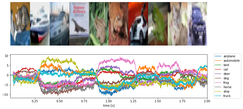
We can see that we have successfully deployed the network we trained onto Loihi. As mentioned in the introduction, this is still a simplified example designed to fit on a single Loihi chip; we could achieve better performance with a larger model. But these same principles should apply to deploying any deep convolutional network onto Loihi.