Learning

This example shows two ways of implementing learning in the context of NengoSPA. It assumes some basic knowledge of learning in Nengo core, so you might want to check out those examples first.

%matplotlib inline

import nengo
import numpy as np
import matplotlib.pyplot as plt
from cycler import cycler

import nengo_spa as spa

seed = 0
rng = np.random.RandomState(seed + 1)

In this example, we will be learning simple associations from fruits (orange, apricot, cherry, apple) to their colors (orange, yellow, red, green). Thus, we will set up vocabularies accordingly and define the desired target associations.

dim = 64
vocab_fruits = spa.Vocabulary(dimensions=dim, pointer_gen=rng)
vocab_colors = spa.Vocabulary(dimensions=dim, pointer_gen=rng)

fruits = ["ORANGE", "APRICOT", "CHERRY", "APPLE"]
vocab_fruits.populate(";".join(fruits))

colors = ["ORANGE", "YELLOW", "RED", "GREEN"]
vocab_colors.populate(";".join(colors))

targets = {
    "ORANGE": "ORANGE",
    "APRICOT": "YELLOW",
    "CHERRY": "RED",
    "APPLE": "GREEN",
}

matplotlib_colors = {
    "ORANGE": "tab:orange",
    "YELLOW": "yellow",
    "RED": "tab:red",
    "GREEN": "tab:green",
}
matplotlib_color_cycle = cycler(
    "color", [matplotlib_colors[k] for k in vocab_colors.keys()]
)

Furthermore, we define some variables:

• length of the learning period,

• the duration each item will be shown before switching to the next one,

• and the total simulation time.

We also define some helper functions to provide the desired inputs to the model.

item_seconds = 0.2
learn_for_seconds = 10 * item_seconds * len(fruits)

run_for_seconds = learn_for_seconds + len(fruits) * item_seconds


def is_recall(t):
    return t > learn_for_seconds


def current_item(t):
    return fruits[int(t // item_seconds) % len(fruits)]


def current_target(t):
    return targets[current_item(t)]

Method 1: Represent the Semantic Pointers in single, large ensembles

The State module in NengoSPA isn’t a single ensemble, but a slightly more complex network to ensure an accurate representation of Semantic Pointers. However, learning connections work between individual ensembles and not whole networks. To implement learning between two SPA State modules, we can configure the modules to produce only single ensembles and connect those with a learning connection.

Two parameters are important for this:

• subdimensions needs to be set to the total dimensionality of the State’s vocabulary,

• represent_cc_identity must be set to False.

The State ensemble itself can then be accessed via the all_ensembles property, which will only have a single element in this case.

with spa.Network() as model:
    # Inputs to the model
    item = spa.Transcode(
        lambda t: vocab_fruits[current_item(t)], output_vocab=vocab_fruits
    )
    target = spa.Transcode(
        lambda t: vocab_colors[current_target(t)], output_vocab=vocab_colors
    )

    # States/ensembles for learning
    # Note that the `error` state may use multiple ensembles.
    pre_state = spa.State(
        vocab_fruits, subdimensions=vocab_fruits.dimensions, represent_cc_identity=False
    )
    post_state = spa.State(
        vocab_colors, subdimensions=vocab_colors.dimensions, represent_cc_identity=False
    )
    error = spa.State(vocab_colors)

    # Setup the item input and error signals
    item >> pre_state
    -post_state >> error
    target >> error

    # Create the learning connection with some randomly initialized weights
    assert len(pre_state.all_ensembles) == 1
    assert len(post_state.all_ensembles) == 1
    learning_connection = nengo.Connection(
        pre_state.all_ensembles[0],
        post_state.all_ensembles[0],
        function=lambda x: np.random.random(vocab_colors.dimensions),
        learning_rule_type=nengo.PES(0.00015),
    )
    nengo.Connection(error.output, learning_connection.learning_rule, transform=-1)

    # Suppress learning in the final iteration to test recall
    is_recall_node = nengo.Node(is_recall)
    for ens in error.all_ensembles:
        nengo.Connection(
            is_recall_node, ens.neurons, transform=-100 * np.ones((ens.n_neurons, 1))
        )

    # Probes to record simulation data
    p_target = nengo.Probe(target.output)
    p_error = nengo.Probe(error.output, synapse=0.01)
    p_post_state = nengo.Probe(post_state.output, synapse=0.01)

with nengo.Simulator(model) as sim:
    sim.run(run_for_seconds)

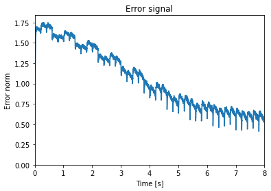
As a sanity check we can look at the norm of the error and see it decrease.

plt.figure()
plt.plot(sim.trange(), np.linalg.norm(sim.data[p_error], axis=1))
plt.xlim(0, learn_for_seconds)
plt.ylim(bottom=0)
plt.title("Error signal")
plt.xlabel("Time [s]")
plt.ylabel("Error norm")

Text(0, 0.5, 'Error norm')

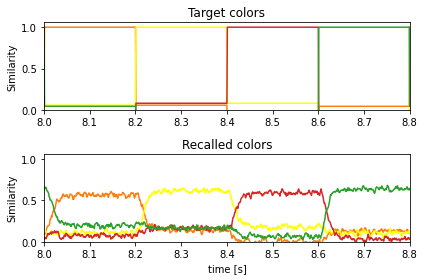
And here is the recall of the learned associations compared to the target colors:

plt.figure()
ax = plt.subplot(2, 1, 1)
ax.set_prop_cycle(matplotlib_color_cycle)
plt.plot(sim.trange(), spa.similarity(sim.data[p_target], vocab_colors))
plt.ylim(bottom=0)
plt.title("Target colors")
plt.ylabel("Similarity")

ax = plt.subplot(2, 1, 2, sharex=ax, sharey=ax)
ax.set_prop_cycle(matplotlib_color_cycle)
plt.plot(sim.trange(), spa.similarity(sim.data[p_post_state], vocab_colors))
plt.xlim(learn_for_seconds, run_for_seconds)
plt.title("Recalled colors")
plt.xlabel("time [s]")
plt.ylabel("Similarity")
plt.tight_layout()

Considerations

This approach allows for full connectivity between the two State modules. Thus, any linear transform could be learned in theory.

However, single ensembles representing large dimensionalities need much more neurons to achieve the same representational accuracy compared to multiple ensembles, where each only represents a subset of all dimensions. Additionally, the model build time and memory usage can be a problem with such large ensembles.

Method 2: Create multiple, pairwise connections between the state ensembles

Instead of configuring the State modules to use only a single ensemble, we can use the default configuration with multiple ensembles and create a separate connection between each pair of ensembles in the pre-synaptic and post-synaptic State. This can be done with a simple for loop and using zip to create the appropriate ensemble pairs. In addition, we need to connect the error signal analogously.

with spa.Network() as model:
    # Inputs to the model
    item = spa.Transcode(
        lambda t: vocab_fruits[current_item(t)], output_vocab=vocab_fruits
    )
    target = spa.Transcode(
        lambda t: vocab_colors[current_target(t)], output_vocab=vocab_colors
    )

    # States/ensembles for learning
    pre_state = spa.State(vocab_fruits)
    post_state = spa.State(vocab_colors)
    error = spa.State(vocab_colors)

    # Setup the item input and error signals
    item >> pre_state
    -post_state >> error
    target >> error

    # Create pairwise learning connections with randomly initialized weights
    for pre_ensemble, post_ensemble, error_ensemble in zip(
        pre_state.all_ensembles, post_state.all_ensembles, error.all_ensembles
    ):
        learning_connection = nengo.Connection(
            pre_ensemble,
            post_ensemble,
            function=lambda x, post_ensemble=post_ensemble: np.random.random(
                post_ensemble.dimensions
            ),
            learning_rule_type=nengo.PES(0.00015),
        )
        nengo.Connection(
            error_ensemble, learning_connection.learning_rule, transform=-1
        )

    # Suppress learning in the final iteration to test recall
    is_recall_node = nengo.Node(is_recall)
    for ens in error.all_ensembles:
        nengo.Connection(
            is_recall_node, ens.neurons, transform=-100 * np.ones((ens.n_neurons, 1))
        )

    # Probes to record simulation data
    p_target = nengo.Probe(target.output)
    p_error = nengo.Probe(error.output, synapse=0.01)
    p_post_state = nengo.Probe(post_state.output, synapse=0.01)

with nengo.Simulator(
    model,
) as sim:
    sim.run(run_for_seconds)

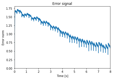
We can look at the error signal again as a sanity check:

plt.figure()
plt.plot(sim.trange(), np.linalg.norm(sim.data[p_error], axis=1))
plt.xlim(0, learn_for_seconds)
plt.ylim(bottom=0)
plt.title("Error signal")
plt.xlabel("Time [s]")
plt.ylabel("Error norm")

Text(0, 0.5, 'Error norm')

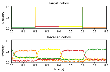
The recall of the learned associations:

plt.figure()
ax = plt.subplot(2, 1, 1)
ax.set_prop_cycle(matplotlib_color_cycle)
plt.plot(sim.trange(), spa.similarity(sim.data[p_target], vocab_colors))
plt.ylim(bottom=0)
plt.title("Target colors")
plt.ylabel("Similarity")

ax = plt.subplot(2, 1, 2, sharex=ax, sharey=ax)
ax.set_prop_cycle(matplotlib_color_cycle)
plt.plot(sim.trange(), spa.similarity(sim.data[p_post_state], vocab_colors))
plt.xlim(learn_for_seconds, run_for_seconds)
plt.title("Recalled colors")
plt.xlabel("time [s]")
plt.ylabel("Similarity")
plt.tight_layout()

Considerations

By using the default ensemble configuration, this approach scales better with regards to build time and representational accuracy. However, the space of potentially learnable functions is limited. Only connectivity matrices with a block diagonal structure can be learned. It is not possible to learn a connection from the \(n\)-th pre-ensemble to the \(m\)-th post-ensemble for \(n \neq m\). This can be fine for certain use cases, such as learning associations, but might not be fine for other use cases. For example, learning the involution is probably not possible with this approach as it requires reversing most of the vector.