
Designing networks
Networks are how Nengo encapsulates functionally complementary objects. Networks can contain ensembles, nodes, connection, even other networks. Models are often made much more readable my grouping objects into networks. Tools for visualizing networks will often use the network structure to produce cleaner images.
Here, we will go over some general principles of network design. In the first section, we will go over these principles with a simple example. In the second section, we will apply these principles to a more complicated example.
Briefly, the general principles we will go over in this tutorial are
Group related objects in networks with
withReuse networks by defining functions
Parameterize functions for more flexible reuse
We will demonstrate these principles with a network consisting of two connected integrators as an example.
[1]:
%matplotlib inline
import matplotlib.pyplot as plt

import nengo
from nengo.dists import Choice
from nengo.processes import Piecewise
from nengo.utils.ipython import hide_input


def test_integrators(net):
    with net:
        piecewise = Piecewise({0: 0, 0.2: 0.5, 1: 0, 2: -1, 3: 0, 4: 1, 5: 0})
        piecewise_inp = nengo.Node(piecewise)
        nengo.Connection(piecewise_inp, net.pre_integrator.input)
        input_probe = nengo.Probe(piecewise_inp)
        pre_probe = nengo.Probe(net.pre_integrator.ensemble, synapse=0.01)
        post_probe = nengo.Probe(net.post_integrator.ensemble, synapse=0.01)
    with nengo.Simulator(net) as sim:
        sim.run(6)
    plt.figure()
    plt.plot(sim.trange(), sim.data[input_probe], color="k")
    plt.plot(sim.trange(), sim.data[pre_probe], color="b")
    plt.plot(sim.trange(), sim.data[post_probe], color="g")


hide_input()
[1]:
1. Group related objects in networks with with
All Nengo objects must be created in the context of some network. We use the with keyword to denote the network context in which a Nengo object is created.
These with statements can be nested to group objects in appropriately named networks.
[2]:
# Example: two connected integrators
#  (See integrator example network for more details)
net = nengo.Network(label="Two integrators")
with net:
    with nengo.Network() as pre_integrator:
        pre_input = nengo.Node(size_in=1)
        pre_ensemble = nengo.Ensemble(100, dimensions=1)
        nengo.Connection(pre_ensemble, pre_ensemble, synapse=0.1)
        nengo.Connection(pre_input, pre_ensemble, synapse=None, transform=0.1)
    with nengo.Network() as post_integrator:
        post_input = nengo.Node(size_in=1)
        post_ensemble = nengo.Ensemble(100, dimensions=1)
        nengo.Connection(post_ensemble, post_ensemble, synapse=0.1)
        nengo.Connection(post_input, post_ensemble, synapse=None, transform=0.1)
    nengo.Connection(pre_ensemble, post_input)
[3]:
# Test the integrators by giving piecewise input and plotting
with net:
piecewise = Piecewise({0: 0, 0.2: 0.5, 1: 0, 2: -1, 3: 0, 4: 1, 5: 0})
piecewise_inp = nengo.Node(piecewise)
nengo.Connection(piecewise_inp, pre_input)
input_probe = nengo.Probe(piecewise_inp)
pre_probe = nengo.Probe(pre_ensemble, synapse=0.01)
post_probe = nengo.Probe(post_ensemble, synapse=0.01)
with nengo.Simulator(net) as sim:
sim.run(6)
plt.figure()
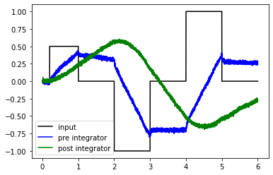
plt.plot(sim.trange(), sim.data[input_probe], color="k", label="input")
plt.plot(sim.trange(), sim.data[pre_probe], color="b", label="pre integrator")
plt.plot(sim.trange(), sim.data[post_probe], color="g", label="post integrator")
plt.legend(loc="best")
[3]:
<matplotlib.legend.Legend at 0x7f05dab030f0>
Note that the with statements are not just cosmetic; Nengo objects are stored in the network that they’re constructed in.
[4]:
assert pre_input in pre_integrator
assert pre_input not in net
assert pre_integrator in net
2. Reuse networks by defining functions
Often, the same network is constructed more than once, resulting in duplicated code. We can reduce this code duplication by defining a function that creates the network and returns it.
Even if you only use the network once, it can be helpful to define all of your subnetworks in functions to keep your code cleaner. Determining when a network should be defined in a function is informed by experience designing large networks and personal preference.
Store useful objects on the network
A corollary to putting networks in functions is that any objects that you might want access to outside of that function should be stored on the network. Functions that create networks should only return that network. While all objects in that network are stored somewhere (e.g., ensembles are stored in a net.ensembles list), that list can be large and difficult to search. Therefore, we recommend storing objects on the network itself to make them accessible outside of the function.
[5]:
# Example: two connected integrators. Now with functions!
def Integrator1():
    with nengo.Network() as integrator:
        integrator.input = nengo.Node(size_in=1)
        integrator.ensemble = nengo.Ensemble(100, dimensions=1)
        nengo.Connection(integrator.ensemble, integrator.ensemble, synapse=0.1)
        nengo.Connection(
            integrator.input, integrator.ensemble, synapse=None, transform=0.1
        )
    return integrator


net = nengo.Network(label="Two integrators")
with net:
    net.pre_integrator = Integrator1()
    net.post_integrator = Integrator1()
    nengo.Connection(net.pre_integrator.ensemble, net.post_integrator.input)
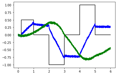
[6]:
# This function does the same as the previous example
test_integrators(net)
3. Parameterize functions for more flexible reuse
Now that your network is created in a function, you can add parameters to your function to change how your network is constructed. This could be a huge change, allowing you to compare two different approaches to some component of your model, or it could something straightforward like changing the number of neurons in the ensembles in the network.
Unlike other languages, Python allows you to add two different types of parameters: positional and keyword arguments. Positional arguments must be passed to your function.
>>> def my_network(arg1, arg2):
...     return f"{arg1} {arg2}"
>>> my_network()
TypeError: my_network() takes exactly 2 arguments (0 given)
>>> my_network(0, 0)
'0 0'
Keyword arguments are assigned a default value, and so do not have to be passed to your function.
>>> def my_network(arg1=0, arg2=0):
...     return f"{arg1} {arg2}"
>>> my_network()
'0 0'
>>> my_network(1)
'1 0'
Order does not matter if you explicitly label the argument in your function call.
>>> my_network(arg2=2, arg1=1)
'1 2'
>>> my_network(arg2=2)
'0 2'
[7]:
# Example: two connected integrators. Functions have parameters!
def Integrator2(n_neurons, dimensions, tau=0.1):
    with nengo.Network() as integrator:
        integrator.input = nengo.Node(size_in=dimensions)
        integrator.ensemble = nengo.Ensemble(n_neurons, dimensions=dimensions)
        nengo.Connection(integrator.ensemble, integrator.ensemble, synapse=tau)
        nengo.Connection(
            integrator.input, integrator.ensemble, synapse=None, transform=tau
        )
    return integrator
[8]:
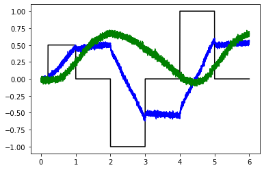
# Try 50 neuron ensembles
net = nengo.Network(label="Two integrators")
with net:
    net.pre_integrator = Integrator2(50, 1)
    net.post_integrator = Integrator2(50, 1)
    nengo.Connection(net.pre_integrator.ensemble, net.post_integrator.input)
test_integrators(net)
[9]:
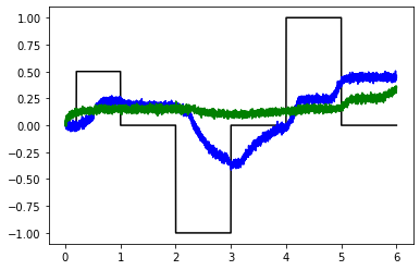
# Try shorter tau (spoiler: it fails to integrate well)
net = nengo.Network(label="Two integrators")
with net:
    net.pre_integrator = Integrator2(50, 1, tau=0.01)
    net.post_integrator = Integrator2(50, 1, tau=0.01)
    nengo.Connection(net.pre_integrator.ensemble, net.post_integrator.input)
test_integrators(net)
Longer example: double integrator network
While the coupled integrator model above seems like a toy example, it is in fact a critical component of many models that capture neurophysiological and behavioral data. Let’s looks at a more complicated network that uses coupled integrators, and show how the network design principles discussed above improve model organization. We will look at a simplified version of the network described in Bekolay et al., 2014.
This network uses two coupled integrators in the context of a simple reaction time task. The subject presses down a lever, and should release that lever between 0.6 and 1.0 seconds later. In order to time the interval, the lever press starts the coupled integrators, which are tuned such that the second integrator should reach a high point by around 0.6 seconds. The second integrator effects the lever release.
We’ll start with a completely disorganized network. Even if you’ve read the paper, the code is quite hard to follow.
[10]:
with nengo.Network() as net:
tau = 0.1
pre_integrator = nengo.Ensemble(200, dimensions=2)
nengo.Connection(
pre_integrator,
pre_integrator[0],
function=lambda x: x[0] * (1.0 - x[1]),
synapse=tau,
)
post_integrator = nengo.Ensemble(200, dimensions=2)
nengo.Connection(
post_integrator,
post_integrator[0],
function=lambda x: x[0] * (1.0 - x[1]),
synapse=tau,
)
nengo.Connection(pre_integrator[0], post_integrator[0], transform=0.16)
press = nengo.Ensemble(
30, dimensions=1, encoders=Choice([[1]]), intercepts=Choice([0.85])
)
release = nengo.Ensemble(
30, dimensions=1, encoders=Choice([[1]]), intercepts=Choice([0.85])
)
nengo.Connection(press, pre_integrator[0], transform=tau * 3)
nengo.Connection(press, post_integrator[1], transform=-1 * 6)
nengo.Connection(post_integrator[0], release)
nengo.Connection(nengo.Node(lambda t: 1 if t < 0.2 else 0), press)
pr_press = nengo.Probe(press, synapse=0.01)
pr_release = nengo.Probe(release, synapse=0.01)
pr_pre_int = nengo.Probe(pre_integrator[0], synapse=0.01)
pr_post_int = nengo.Probe(post_integrator[0], synapse=0.01)
def test_doubleintegrator(net):
with nengo.Simulator(net) as sim:
sim.run(1.4)
t = sim.trange()
plt.figure()
plt.subplot(2, 1, 1)
plt.plot(t, sim.data[pr_press], c="b", label="Press")
plt.plot(t, sim.data[pr_release], c="g", label="Release")
plt.axvspan(0, 0.2, color="b", alpha=0.3)
plt.axvspan(0.8, 1.2, color="g", alpha=0.3)
plt.xlim(right=1.4)
plt.legend(loc="best")
plt.subplot(2, 1, 2)
plt.plot(t, sim.data[pr_pre_int], label="Pre Integrator")
plt.plot(t, sim.data[pr_post_int], label="Post Integrator")
plt.xlim(right=1.4)
plt.legend(loc="best")
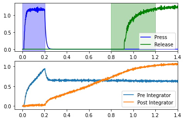
test_doubleintegrator(net)
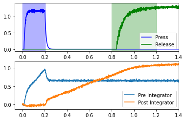
Recall that the goal is to release the lever 0.6-1.0 seconds after the press. The blue “Press” line in the upper plot represents the activity of neurons in motor cortex which effect the lever press. If we assume that the press occurs at 0.2 seconds, then the release window is between 0.8 and 1.2 seconds (shown in green). This will occur if the “Post Integrator” (see lower plot) is sufficiently high during this window. If you rerun the cell above several times, you can see that it usually achieves this, but not all of the time.
Looking at the code, it’s difficult to tell how we achieve this result. It’s also difficult to see what parameters needed tweaking. Rather than just showing one parameter set that works, we should investigate reasonable ranges for each parameter. It would be easy to think that there is only one parameter, tau, in the model as presented, but this is not the case.
Let’s start with the first network design principle: group objects into networks with with.
[11]:
with nengo.Network() as net:
tau = 0.1
with nengo.Network() as mpfc:
with nengo.Network() as pre_integrator:
pre_ensemble = nengo.Ensemble(200, dimensions=2)
nengo.Connection(
pre_ensemble,
pre_ensemble[0],
function=lambda x: x[0] * (1.0 - x[1]),
synapse=tau,
)
with nengo.Network() as post_integrator:
post_ensemble = nengo.Ensemble(200, dimensions=2)
nengo.Connection(
post_ensemble,
post_ensemble[0],
function=lambda x: x[0] * (1.0 - x[1]),
synapse=tau,
)
nengo.Connection(pre_ensemble[0], post_ensemble[0], transform=0.16)
with nengo.Network() as motor:
press = nengo.Ensemble(
30, dimensions=1, encoders=Choice([[1]]), intercepts=Choice([0.85])
)
release = nengo.Ensemble(
30, dimensions=1, encoders=Choice([[1]]), intercepts=Choice([0.85])
)
nengo.Connection(press, pre_ensemble[0], transform=tau * 3)
nengo.Connection(press, post_ensemble[1], transform=-1 * 6)
nengo.Connection(post_ensemble[0], release)
nengo.Connection(nengo.Node(lambda t: 1 if t < 0.2 else 0), press)
pr_press = nengo.Probe(press, synapse=0.01)
pr_release = nengo.Probe(release, synapse=0.01)
pr_pre_int = nengo.Probe(pre_ensemble[0], synapse=0.01)
pr_post_int = nengo.Probe(post_ensemble[0], synapse=0.01)
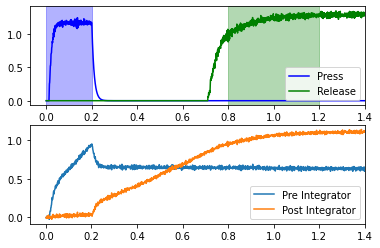
test_doubleintegrator(net)
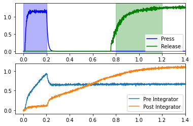
This exhibits some of the hypotheses of this model; specifically, that the medial prefrontal cortex contains these integrators, and that they can be involved in control of motor actions.
Let’s do both of the remaining principles by making some parameterized functions to get a sense of all of the knobs that be be tweaked in this model.
[12]:
def controlled_integrator(n_neurons, dimensions, tau=0.1):
    with nengo.Network() as integrator:
        integrator.ensemble = nengo.Ensemble(n_neurons, dimensions=dimensions + 1)
        nengo.Connection(
            integrator.ensemble,
            integrator.ensemble[:dimensions],
            function=lambda x: x[:-1] * (1.0 - x[-1]),
            synapse=tau,
        )
    return integrator


def medial_pfc(coupling_strength, n_neurons_per_integrator=200, tau=0.1):
    with nengo.Network() as medial_pfc:
        medial_pfc.pre = controlled_integrator(n_neurons_per_integrator, 1, tau)
        medial_pfc.post = controlled_integrator(n_neurons_per_integrator, 1, tau)
        nengo.Connection(
            medial_pfc.pre.ensemble[0],
            medial_pfc.post.ensemble[0],
            transform=coupling_strength,
        )
    return medial_pfc


def motor_cortex(command_threshold, n_neurons_per_command=30):
    with nengo.Network() as motor_cortex:
        ens_args = {
            "dimensions": 1,
            "encoders": Choice([[1]]),
            "intercepts": Choice([command_threshold]),
        }
        motor_cortex.press = nengo.Ensemble(n_neurons_per_command, **ens_args)
        motor_cortex.release = nengo.Ensemble(n_neurons_per_command, **ens_args)
    return motor_cortex


def double_integrator(
    mpfc_coupling_strength,
    command_threshold,
    press_to_pre_gain=3,
    press_to_post_control=-6,
    recurrent_tau=0.1,
    seed=None,
):
    with nengo.Network(seed=seed) as net:
        net.mpfc = medial_pfc(mpfc_coupling_strength)
        net.motor = motor_cortex(command_threshold)
        nengo.Connection(
            net.motor.press,
            net.mpfc.pre.ensemble[0],
            transform=recurrent_tau * press_to_pre_gain,
        )
        nengo.Connection(
            net.motor.press, net.mpfc.post.ensemble[1], transform=press_to_post_control
        )
        nengo.Connection(net.mpfc.post.ensemble[0], net.motor.release)
    return net


def test_doubleintegrator_wprobes(net):
    # Provide input and probe outside of network construction,
    # for more flexibility
    with net:
        nengo.Connection(nengo.Node(lambda t: 1 if t < 0.2 else 0), net.motor.press)
        pr_press = nengo.Probe(net.motor.press, synapse=0.01)
        pr_release = nengo.Probe(net.motor.release, synapse=0.01)
        pr_pre_int = nengo.Probe(net.mpfc.pre.ensemble[0], synapse=0.01)
        pr_post_int = nengo.Probe(net.mpfc.post.ensemble[0], synapse=0.01)
    with nengo.Simulator(net) as sim:
        sim.run(1.4)
    t = sim.trange()
    plt.figure()
    plt.subplot(2, 1, 1)
    plt.plot(t, sim.data[pr_press], c="b", label="Press")
    plt.plot(t, sim.data[pr_release], c="g", label="Release")
    plt.axvspan(0, 0.2, color="b", alpha=0.3)
    plt.axvspan(0.8, 1.2, color="g", alpha=0.3)
    plt.xlim(right=1.4)
    plt.legend(loc="best")
    plt.subplot(2, 1, 2)
    plt.plot(t, sim.data[pr_pre_int], label="Pre Integrator")
    plt.plot(t, sim.data[pr_post_int], label="Post Integrator")
    plt.xlim(right=1.4)
    plt.legend(loc="best")


net = double_integrator(mpfc_coupling_strength=0.16, command_threshold=0.85)
test_doubleintegrator_wprobes(net)
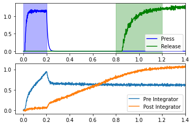
While this does add some complexity and length, the effort is worth it, as we can now do simple parameters sweeps to investigate the effects of changing various parameters.
[13]:
for coupling_strength in (0.11, 0.16, 0.21):
    net = double_integrator(
        mpfc_coupling_strength=coupling_strength, command_threshold=0.85, seed=0
    )
    test_doubleintegrator_wprobes(net)
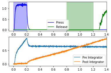
The coupling_strength changes how quickly the “Post Integrator” rises, which causes the release to occur at different times. Of the values tested, only a coupling strength of 0.16 effects the release during the release window (for this particular network seed).
We will looks at some more techniques for cleaning up this network code and making it more flexible in “Additional tips and tricks for designing networks”.