
- Introduction
- Installation
- User guide
- API reference
- Examples
- Coming from Nengo to NengoDL
- Coming from TensorFlow to NengoDL
- Integrating a Keras model into a Nengo network
- Optimizing a spiking neural network
- Converting a Keras model to a spiking neural network
- Legendre Memory Units in NengoDL
- Optimizing a cognitive model
- Optimizing a cognitive model with temporal dynamics
- Additional resources
- Project information
Coming from TensorFlow to NengoDL
![]()
NengoDL combines two frameworks: Nengo and TensorFlow. This tutorial is designed for people who are familiar with TensorFlow and looking to learn more about neuromorphic modelling with NengoDL. For the other approach, users familiar with Nengo looking to learn how to use NengoDL, check out this tutorial.
If you are familiar with Keras you may also be interested in KerasSpiking, a companion project to NengoDL that has a more minimal feature set, but integrates even more transparently with the Keras API. See this page for a more detailed comparison between the two projects.
[1]:
%matplotlib inline

import warnings

import matplotlib.pyplot as plt
import nengo
from nengo.utils.matplotlib import rasterplot
import numpy as np
import tensorflow as tf

import nengo_dl


warnings.simplefilter("ignore")
tf.get_logger().addFilter(lambda rec: "Tracing is expensive" not in rec.msg)
What is Nengo
We’ll start with the very basics, where you might be wondering what Nengo is and why you would want to use it. Nengo is a tool for constructing and simulating neural networks. That is, to some extent, the same purpose as TensorFlow (and its higher level API, Keras). For example, here is how we might build a simple two layer auto-encoder network in TensorFlow:
[2]:
n_in = 784
n_hidden = 64
minibatch_size = 50

# input
tf_a = tf.keras.Input(shape=(n_in,))

# first layer
tf_b = tf.keras.layers.Dense(
    n_hidden, activation=tf.nn.relu, kernel_initializer=tf.initializers.glorot_uniform()
)(tf_a)

# second layer
tf_c = tf.keras.layers.Dense(
    n_in, activation=tf.nn.relu, kernel_initializer=tf.initializers.glorot_uniform()
)(tf_b)
And here is how we would build the same network architecture in Nengo:
[3]:
with nengo.Network() as auto_net:
    # input
    nengo_a = nengo.Node(np.zeros(n_in))

    # first layer
    nengo_b = nengo.Ensemble(n_hidden, 1, neuron_type=nengo.RectifiedLinear())
    nengo.Connection(nengo_a, nengo_b.neurons, transform=nengo_dl.dists.Glorot())

    # second layer
    nengo_c = nengo.Ensemble(n_in, 1, neuron_type=nengo.RectifiedLinear())
    nengo.Connection(
        nengo_b.neurons, nengo_c.neurons, transform=nengo_dl.dists.Glorot()
    )

    # probes are used to collect data from the network
    p_c = nengo.Probe(nengo_c.neurons)
One difference you’ll note is that with Nengo we separate the creation of the layers and the creation of the connections between layers. This is because the connection structure in Nengo networks often has a lot more state and general complexity than in typical deep learning networks, so it is helpful to be able to control it independently (we’ll see examples of this later).
Another new object you may notice is the nengo.Probe. This is used to collect data from the simulation; by adding a probe to nengo_c.neurons, we are indicating that we want to collect the activities of those neurons when the simulation is running. You can think of this like the outputs arguments in a Keras Model.
We will not go into a lot of detail on Nengo here; there is much more functionality available, but we will focus on the features most familiar or relevant to those coming from a TensorFlow background. For a more in-depth introduction to Nengo, check out the Nengo-specific documentation and examples.
Simulating a network
To simulate a Keras network we create a Model and call model.predict:
[4]:
model = tf.keras.Model(inputs=tf_a, outputs=tf_c)
out = model.predict(np.ones((minibatch_size, n_in)))
print(out.shape)
2/2 [==============================] - 0s 3ms/step
(50, 784)
Again, accomplishing the same thing in Nengo bears many similarities. We create a Simulator and call sim.predict:
[5]:
with nengo_dl.Simulator(network=auto_net, minibatch_size=minibatch_size) as sim:
    out = sim.predict(np.ones((minibatch_size, 1, n_in)))
    print(out[p_c].shape)
Build finished in 0:00:00
Optimization finished in 0:00:00
Construction finished in 0:00:00
1/1 [==============================] - 0s 283ms/step
(50, 1, 784)
One difference you may note is the extra dimension with size 1 in the shape of the Nengo inputs and outputs. This represents the time dimension; in this example we’re only running for a single timestep, which is why it has size 1, but this could be used to provide different input values on each simulation timestep.
This highlights a key difference between Nengo and TensorFlow. Nengo simulations are fundamentally temporal in nature; unlike TensorFlow where the graph simply represents an abstract set of computations, in Nengo we (almost) always think of the graph as representing a stateful neural simulation, where values are accumulated, updated, and communicated over time. This is not to say there is no overlap (we can create TensorFlow simulations that execute over time, and we can create Nengo simulations without temporal dynamics), but this is a different way of thinking about computations that influences how we construct and simulate networks in Nengo.
More details on the NengoDL Simulator can be found in the user guide.
Spiking networks
Although Nengo can be used to create TensorFlow-style networks, it has been primarily designed for a different style of modelling: “neuromorphic” networks. Neuromorphic networks include features drawn from biological neural networks, in an effort to understand or recreate the functionality of biological brains. Note that these models fall on a spectrum with standard artificial neural networks, with different approaches incorporating different biological features. But in general the structure and parameterization of these networks often differs significantly from standard deep network architectures.
We touched on this above in the discussion of temporality, which is one common feature of neuromorphic networks. Another common characteristic is the use of more complicated neuron models, in particular spiking neurons. In contrast to “rate” neurons (like relu) that output a continuous value, spiking neurons communicate via discrete bursts of output called spikes.
We can visualize this difference with a simple 1-layer network. In this example we’ll use sim.run_steps to run the simulation, rather than sim.predict. sim.run_steps (or sim.run) is a standard Nengo Simulator execution function (as opposed to sim.predict, which is specific to NengoDL). We could use either one, but you will probably see sim.run in Nengo code, so we introduce it here. The main difference in this case is that results will be stored in the sim.data
dictionary, as opposed to being returned directly from sim.predict.
[6]:
with nengo.Network() as net:
# our input node will output a sine wave with a period of 1 second
a = nengo.Node(lambda t: np.sin(2 * np.pi * t))
# we'll create one ensemble with rate neurons
b_rate = nengo.Ensemble(10, 1, neuron_type=nengo.RectifiedLinear(), seed=2)
nengo.Connection(a, b_rate)
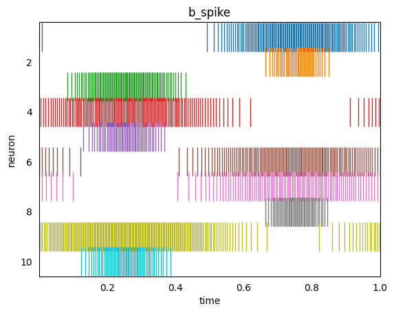
# and another ensemble with spiking neurons
b_spike = nengo.Ensemble(10, 1, neuron_type=nengo.SpikingRectifiedLinear(), seed=2)
nengo.Connection(a, b_spike)
p_a = nengo.Probe(a)
p_rate = nengo.Probe(b_rate.neurons)
p_spike = nengo.Probe(b_spike.neurons)
with nengo_dl.Simulator(net) as sim:
# simulate the model for 1 second
# note that we are not providing any input data, so input
# data will be automatically generated based on the sine function
# in the Node definition.
sim.run_steps(1000)
plt.figure()
plt.plot(sim.trange(), sim.data[p_a])
plt.xlabel("time")
plt.ylabel("input value")
plt.title("a")
plt.figure()
plt.plot(sim.trange(), sim.data[p_rate])
plt.xlabel("time")
plt.ylabel("firing rate")
plt.title("b_rate")
plt.figure()
rasterplot(sim.trange(), sim.data[p_spike])
plt.xlabel("time")
plt.ylabel("neuron")
plt.title("b_spike")
plt.show()
Build finished in 0:00:00
Optimization finished in 0:00:00
Construction finished in 0:00:00
Simulation finished in 0:00:00
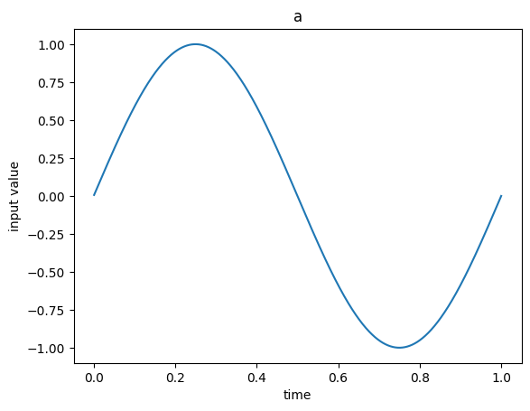
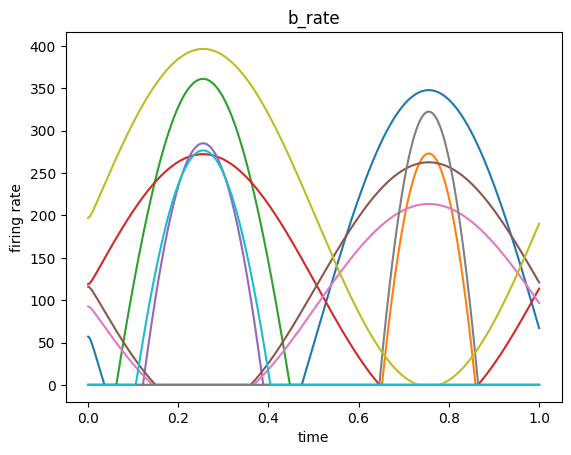
Each neuron responds to the input signal differently due to the random parameterization in the network (e.g. connection weights and biases). We have matched the parameterization in the rate and spiking ensembles so that it is easier to see the parallels.
Note that the same information is being represented in the two ensembles. For example, when the second neuron (orange) is outputting a high continuous value (in the second graph), the corresponding spiking neuron is outputting more discrete spikes (orange lines in the third graph).
We can see the parallels more clearly if we introduce another Nengo feature, synaptic filters. This is inspired by a biological feature where discrete spikes induce a continuous electrical waveform in the receiving neuron, at the synapse (the point where the two neurons connect). But computationally we can think of this simply as applying a filter to the spiking signal.
[7]:
# nengo uses a linear lowpass filter by default
filt = nengo.Lowpass(tau=0.05)

# apply filter to ensemble output spikes
filtered_spikes = filt.filt(sim.data[p_spike])

plt.figure()
plt.plot(sim.trange(), filtered_spikes)
plt.xlabel("time")
plt.ylabel("filtered spike train (firing rates)")
plt.show()
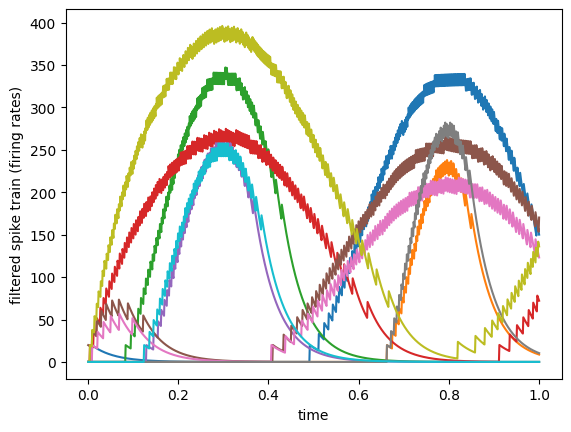
We can see how the spike trains, when viewed through a synaptic filter, approximate the continuous rate values in the second graph above.
In this example we have computed the filtered signal manually for demonstration purposes, but in a typical Nengo model these synaptic filters are applied throughout the model, on the Connection objects. For example, the above filtering would be equivalent to nengo.Connection(b_spike.neurons, x, synapse=0.05) (from the perspective of a hypothetical downstream object x).
This is a helpful duality to keep in mind when coming to neuromorphic modelling and Nengo from a standard deep network background. Although spiking neurons seem like a radically different paradigm, they can compute and communicate the same information as their rate counterparts. But note that this only makes sense when we think of the network temporally (neurons spiking and being filtered over time).
There are many other neuron types built into Nengo (see the documentation for a complete list). These neuron models have various different behaviours, and managing their parameterization and simulation is an important part of Nengo’s design.
Inserting TensorFlow code
The goal of NengoDL is not to replace TensorFlow or Nengo, but to allow them to smoothly work together. Thus one important feature is the ability to write TensorFlow code directly, and insert it into a Nengo network. This allows us to use whichever framework is best suited for different parts of a model.
This functionality is accessed through the nengo_dl.TensorNode class. This allows us to wrap TensorFlow code in a Nengo object, so that it can easily communicate with the rest of a Nengo model. The TensorFlow code is written in a function that takes tf.Tensors as input, applies the desired manipulations through TensorFlow operations, and returns a tf.Tensor. We then pass that function to the TensorNode.
For simple cases we can use nengo_dl.Layer. This is a simplified interface for constructing TensorNodes that mimics the Keras functional API. For example, suppose we want to apply batch normalization to the output of one of the Nengo ensembles. There is no built-in way to do batch normalization in Nengo, so we can instead turn to TensorFlow for this part of the model.
[8]:
with net:
    batch_norm = nengo_dl.Layer(tf.keras.layers.BatchNormalization(momentum=0.9))(
        b_rate.neurons
    )
    p_batch_norm = nengo.Probe(batch_norm)
This is essentially equivalent to the Keras layer tf.keras.layers.BatchNormalization, except it works with Nengo objects. For example, b_rate is a nengo.Ensemble in this case, and we can add Probes or Connections to batch_norm in the same way as any other Nengo object.
Using nengo_dl.Layer is simply a shortcut for creating a TensorNode and Connection; the above is equivalent to
[9]:
with net:
    batch_norm = nengo_dl.TensorNode(
        tf.keras.layers.BatchNormalization(momentum=0.9),
        shape_in=(10,),
        pass_time=False,
    )
    nengo.Connection(b_rate.neurons, batch_norm, synapse=None)
    p_batch_norm = nengo.Probe(batch_norm)
In general, we can use any function (a built in TensorFlow function or one we write ourselves) in a TensorNode. It can accept two parameters, t and x, where t is the current simulation time and x is the value of any Connections incoming to the TensorNode. We can use pass_time=False if we don’t need the time input. x will have shape (minibatch_size,) + shape_in, where shape_in is the parameter passed to the TensorNode (or inferred from the input object in the
case of nengo_dl.Layer). The TensorNode/Layer function should return a tf.Tensor with shape (minibatch_size,) + shape_out, where shape_out is the output dimensionality of the node (dependent on the manipulations applied to the inputs x). We could explicitly specify shape_out=(10,) in the above example, or if we don’t specify the output shape it will be determined automatically by calling the node function with placeholder inputs.
Here is a simple network to illustrate a TensorNode’s input and output:
[10]:
with nengo.Network() as net:
    # node to provide an input value for the TensorNode
    a = nengo.Node([0.5, -0.1])

    # a TensorNode function to illustrate i/o
    def tensor_func(t, x):
        # print out the value of inputs t and x
        print_t = tf.print("t:", t)
        with tf.control_dependencies([print_t]):
            print_x = tf.print("x:", x)

        # output t + x
        with tf.control_dependencies([print_x]):
            return tf.add(t, x)

    # create the TensorNode
    b = nengo_dl.TensorNode(tensor_func, shape_in=(2,), shape_out=(2,))
    nengo.Connection(a, b, synapse=None)

    p = nengo.Probe(b)

with nengo_dl.Simulator(net) as sim:
    print("TensorNode input:")
    data = sim.predict(n_steps=10)
    print("TensorNode output:")
    print(data[p])
Build finished in 0:00:00
Optimization finished in 0:00:00
Construction finished in 0:00:00
TensorNode input:
t: 0.001
x: [[0.5 -0.1]]
t: 0.002
x: [[0.5 -0.1]]
t: 0.003
x: [[0.5 -0.1]]
t: 0.004
x: [[0.5 -0.1]]
t: 0.00500000035
x: [[0.5 -0.1]]
t: 0.006
x: [[0.5 -0.1]]
t: 0.007
x: [[0.5 -0.1]]
t: 0.008
x: [[0.5 -0.1]]
t: 0.00900000054
x: [[0.5 -0.1]]
t: 0.0100000007
x: [[0.5 -0.1]]
1/1 [==============================] - 0s 156ms/step
TensorNode output:
[[[ 0.501 -0.099]
  [ 0.502 -0.098]
  [ 0.503 -0.097]
  [ 0.504 -0.096]
  [ 0.505 -0.095]
  [ 0.506 -0.094]
  [ 0.507 -0.093]
  [ 0.508 -0.092]
  [ 0.509 -0.091]
  [ 0.51  -0.09 ]]]
We can see, as we expect, that the input tensor t is reflecting the current simulation time over the 10 timesteps we executed, and x contains the value of the input Node that we connected to the TensorNode. And we can see in the probe data that the TensorNode is outputting the operation we defined in TensorFlow (tf.add(t, x)).
We can define more complicated TensorNodes by implementing a custom Keras Layer. This can be useful, for example, if the TensorNode requires internal parameters (which should be created in the Keras Layer’s build function).
Here is a simple TensorNode that illustrates the usage of a custom Layer:
[11]:
with nengo.Network() as net:

    class MyLayer(tf.keras.layers.Layer):
        def build(self, input_shape):
            self.w = self.add_weight(shape=(1, 1))

        def call(self, inputs):
            return inputs * self.w

    a = nengo_dl.TensorNode(MyLayer(), shape_in=(1,), pass_time=False)
More details on TensorNode usage can be found in the user guide.
Deep learning parameter optimization
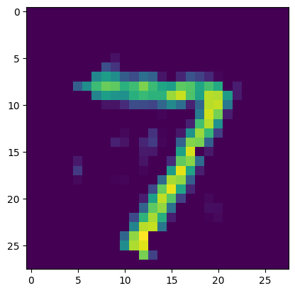
NengoDL allows model parameters to be optimized via TensorFlow optimization algorithms, through the Simulator.fit function. Returning to the autoencoder examples from the beginning of this tutorial, we’ll optimize those networks to encode MNIST digits.
[12]:
# download MNIST dataset
(train_data, _), (test_data, _) = tf.keras.datasets.mnist.load_data()
# flatten images
train_data = train_data.reshape((train_data.shape[0], -1))
test_data = test_data.reshape((test_data.shape[0], -1))

n_epochs = 2
In TensorFlow the training would be done something like:
[13]:
model = tf.keras.Model(inputs=tf_a, outputs=tf_c)
model.compile(optimizer=tf.optimizers.RMSprop(1e-3), loss=tf.losses.mse)

# run training loop
model.fit(train_data, train_data, epochs=n_epochs)

# evaluate performance on test set
model.evaluate(test_data, test_data)

# display example output
output = model.predict(test_data[[0]])
plt.figure()
plt.imshow(output[0].reshape((28, 28)))
plt.show()
Epoch 1/2
1875/1875 [==============================] - 4s 2ms/step - loss: 1286.3943
Epoch 2/2
1875/1875 [==============================] - 3s 2ms/step - loss: 944.7948
313/313 [==============================] - 1s 1ms/step - loss: 923.4284
1/1 [==============================] - 0s 41ms/step
Before running the same training in NengoDL, we’ll change the Nengo model parameters to more closely match the TensorFlow network (we omitted these details in the original presentation to keep things simple).
[14]:
# set initial neuron gains to 1 and biases to 0
for ens in auto_net.all_ensembles:
    ens.gain = nengo.dists.Choice([1])
    ens.bias = nengo.dists.Choice([0])

# disable synaptic filtering on all connections
for conn in auto_net.all_connections:
    conn.synapse = None
We also need to modify the data slightly. As mentioned above, NengoDL simulations are essentially temporal, so data is described over time (indicating what the inputs/targets should be on each simulation timestep). So instead of the data having shape (batch_size, n), it will have shape (batch_size, n_steps, n). In this case we’ll just be training for a single timestep, but we still need to add that extra axis with length 1.
[15]:
train_data = train_data[:, None, :]
test_data = test_data[:, None, :]
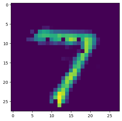
Now we can run the NengoDL equivalent of the above TensorFlow training (note: the results will not match exactly due to different random initializations):
[16]:
with nengo_dl.Simulator(auto_net, minibatch_size=minibatch_size) as sim:
    sim.compile(optimizer=tf.optimizers.RMSprop(1e-3), loss=tf.losses.mse)

    # run training loop
    sim.fit(train_data, train_data, epochs=n_epochs)

    # evaluate performance on test set
    sim.evaluate(test_data, test_data)

    # display example output
    output = sim.predict(test_data[:minibatch_size])
    plt.figure()
    plt.imshow(output[p_c][0].reshape((28, 28)))
    plt.show()
Build finished in 0:00:00
Optimization finished in 0:00:00
Construction finished in 0:00:00
Epoch 1/2
1200/1200 [==============================] - 6s 4ms/step - loss: 1376.8668 - probe_loss: 1376.8668
Epoch 2/2
1200/1200 [==============================] - 5s 4ms/step - loss: 936.0474 - probe_loss: 936.0474
  1/200 [..............................] - ETA: 50s - loss: 767.3197 - probe_loss: 767.3197WARNING:tensorflow:Callback method `on_test_batch_end` is slow compared to the batch time (batch time: 0.0013s vs `on_test_batch_end` time: 0.0015s). Check your callbacks.
WARNING:tensorflow:Callback method `on_test_batch_end` is slow compared to the batch time (batch time: 0.0013s vs `on_test_batch_end` time: 0.0015s). Check your callbacks.
200/200 [==============================] - 1s 3ms/step - loss: 875.5232 - probe_loss: 875.5232
1/1 [==============================] - 0s 208ms/step
More details on using sim.fit can be found in the user guide.
NEF parameter optimization
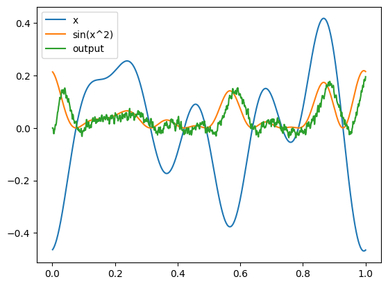
NengoDL also provides access to a different optimization method, the Neural Engineering Framework (NEF). This uses linear least-squares optimization to solve for optimal connection weights analytically, rather than using an iterative gradient-descent based algorithm. The advantage of the NEF is that it is very fast and general (for example, it does not require the network to be differentiable). The disadvantage is that it optimizes each set of connection weights individually (i.e., it cannot jointly optimize across multiple layers).
The NEF optimization is accessed by setting the function argument on a nengo.Connection. This specifies the function that we would like those connection weights to approximate. In addition, in previous examples you may have noticed that we were forming Connections using ensemble.neurons (rather than ensemble). Using ensemble.neurons specifies that we want to form a direct connection between ensemble neurons, without applying the NEF optimization. So when we want to use the
function argument, the Connection source object should be an ensemble, not ensemble.neurons. For example, we could use the NEF to create a network to approximate the function \(sin(x^2)\):
[17]:
with nengo.Network(seed=0) as net:
    # input node outputting a random signal for x
    inpt = nengo.Node(nengo.processes.WhiteSignal(1, 5, rms=0.3))

    # first ensemble, will compute x^2
    ens0 = nengo.Ensemble(50, 1)

    # second ensemble, will compute sin(x^2)
    ens1 = nengo.Ensemble(50, 1)

    # output node
    outpt = nengo.Node(size_in=1)

    # connect input to first ensemble
    nengo.Connection(inpt, ens0)

    # connect first to second ensemble, solve for weights
    # to approximate the square function
    nengo.Connection(ens0, ens1, function=np.square)

    # connect second ensemble to output, solve for weights
    # to approximate the sin function
    nengo.Connection(ens1, outpt, function=np.sin)

    # add a probe on the input and output
    inpt_p = nengo.Probe(inpt)
    outpt_p = nengo.Probe(outpt, synapse=0.005)

with nengo_dl.Simulator(net, seed=0) as sim:
    sim.run_steps(1000)

plt.figure()
plt.plot(sim.trange(), sim.data[inpt_p], label="x")
plt.plot(sim.trange(), np.sin(sim.data[inpt_p] ** 2), label="sin(x^2)")
plt.plot(sim.trange(), sim.data[outpt_p], label="output")
plt.legend()
plt.show()
Build finished in 0:00:00
Optimization finished in 0:00:00
Construction finished in 0:00:00
Simulation finished in 0:00:00

The NEF optimization can be used in combination with the deep learning optimization methods. For example, we could optimize some parameters with the NEF and others with sim.fit (see this example). Or we could initialize each set of connection weights individually with the NEF, and then further refine them with end-to-end training via sim.fit. As always, the overall theme is that NengoDL allows us to use whichever method is most
appropriate for a particular goal.
See this example for a deeper introduction to the principles of the NEF.
Running on neuromorphic hardware
Neuromorphic hardware is specialized compute hardware designed to simulate neuromorphic networks quickly/efficiently. However, often it is difficult to program this custom hardware, and it requires writing custom code for each neuromorphic platform. One of the primary design goals of Nengo is to alleviate these challenges, by providing a single API that can be used to build networks across many different neuromorphic platforms.
The idea is that the front-end network construction code is the same (Networks, Nodes, Ensembles, Connections, and Probes), and then each platform has its own Simulator class (the back-end) that compiles and executes that network definition for some compute platform. This provides a consistent interface so that we only need to write code once and can then run that network on novel hardware platforms with no additional effort. For example, we could take the network from
above and simulate it on different hardware platforms:
[18]:
# run on a standard CPU
with nengo.Simulator(net, seed=0) as sim:
    sim.run_steps(1000)

# run on Loihi neuromorphic hardware
# (requires https://www.nengo.ai/nengo-loihi/)
# with nengo_loihi.Simulator(net, seed=0) as sim:
#     sim.run_steps(1000)

# run on SpiNNaker neuromorphic hardware
# (requires https://github.com/project-rig/nengo_spinnaker)
# with nengo_spinnaker.Simulator(net, seed=0) as sim:
#     sim.run_steps(1000)

# run on any OpenCL-compatible hardware
# (requires https://github.com/nengo-labs/nengo-ocl)
# with nengo_ocl.Simulator(net, seed=0) as sim:
#     sim.run_steps(1000)

plt.figure()
plt.plot(sim.trange(), sim.data[inpt_p], label="x")
plt.plot(sim.trange(), np.sin(sim.data[inpt_p] ** 2), label="sin(x^2)")
plt.plot(sim.trange(), sim.data[outpt_p], label="output")
plt.legend()
plt.show()
We have commented out the different backends above because they require extra installation steps, but if you are running this example yourself you can install any of those backends (or more) and uncomment that code to see the same network running on that new hardware platform. Note that we can think of NengoDL as a TensorFlow back-end (among other things); it takes a standard Nengo network, and simulates it using TensorFlow.
We can take advantage of this cross-platform compatibility to effectively incorporate NengoDL’s deep learning functionality into any other Nengo back-end. We build our Network, optimize it in NengoDL, save the optimized model parameters back into the Network definition, and then simulate that optimized Network in a different back-end. See this example in nengo-loihi, where a spiking network is optimized in NengoDL and then deployed on Loihi.
Conclusion
In this tutorial we have demonstrated how to translate TensorFlow concepts into NengoDL, including network construction, execution, and optimization. We have also discussed how to use TensorNodes to combine TensorFlow and Nengo code, and introduced some of the unique features of Nengo (such as NEF optimization and neuromorphic cross-platform execution). However, there is much more functionality in NengoDL than we are able to introduce here; check out the user guide or other examples for more information. If you would like more information on how NengoDL is implemented under the hood using TensorFlow, check out the white paper.