Optimizing a spiking neural network

Almost all deep learning methods are based on gradient descent, which means that the network being optimized needs to be differentiable. Deep neural networks are usually built using rectified linear or sigmoid neurons, as these are differentiable nonlinearities. However, in neurmorphic modelling we often want to use spiking neurons, which are not differentiable. So the challenge is how to apply deep learning methods to spiking neural networks.

A method for accomplishing this is presented in Hunsberger and Eliasmith (2016). The basic idea is to use a differentiable approximation of the spiking neurons during the training process, and the actual spiking neurons during inference. NengoDL will perform these transformations automatically if the user tries to optimize a model containing a spiking neuron model that has an equivalent, differentiable rate-based implementation. In this example we will use these techniques to develop a network to classify handwritten digits (MNIST) in a spiking convolutional network.

%matplotlib inline

from urllib.request import urlretrieve

import nengo
import tensorflow as tf
import numpy as np
import matplotlib.pyplot as plt

import nengo_dl

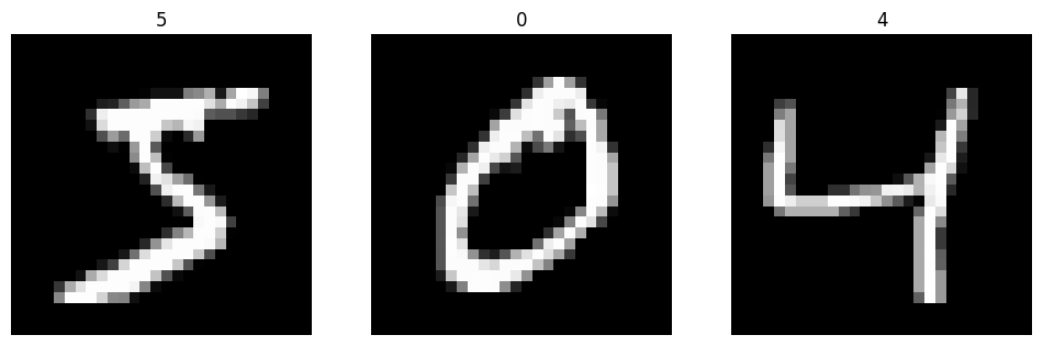
First we’ll load the training data, the MNIST digits/labels.

(train_images, train_labels), (
    test_images,
    test_labels,
) = tf.keras.datasets.mnist.load_data()

# flatten images
train_images = train_images.reshape((train_images.shape[0], -1))
test_images = test_images.reshape((test_images.shape[0], -1))

plt.figure(figsize=(12, 4))
for i in range(3):
    plt.subplot(1, 3, i + 1)
    plt.imshow(np.reshape(train_images[i], (28, 28)), cmap="gray")
    plt.axis("off")
    plt.title(str(train_labels[i]))

Next we’ll build a simple convolutional network. This architecture is chosen to be a quick and easy solution for this task; other tasks would likely require a different architecture, but the same general principles will apply.

We will use TensorNodes to construct the network, as they allow us to directly insert TensorFlow code into Nengo. We could use native Nengo objects instead, but in this example we’ll use TensorNodes to make the parallels with standard deep networks as clear as possible. To make things even easier, we’ll use nengo_dl.Layer. This is a utility function for constructing TensorNodes that mimics the Keras functional API.

nengo_dl.Layer is used to build a sequence of layers, where each layer takes the output of the previous layer and applies some transformation to it. When working with TensorFlow’s Keras API, we can create Keras Layers and then simply pass those layer objects to nengo_dl.Layer to encapsulate them in a TensorNode.

Normally all signals in a Nengo model are (batched) vectors. However, certain layer functions, such as convolutional layers, may expect a different shape for their inputs. If the shape_in argument is specified when applying a Layer to some input, then the inputs will automatically be reshaped to the given shape. Note that this shape does not include the batch dimension on the first axis, as that will be set automatically by the simulation.

Layer can also be passed a Nengo NeuronType, instead of a Tensor function. In this case Layer will construct an Ensemble implementing the given neuron nonlinearity (the rest of the arguments work the same).

Note that Layer is just a syntactic wrapper for constructing TensorNodes or Ensembles; anything we build with a Layer we could instead construct directly using those underlying components. Layer just simplifies the construction of this common layer-based pattern. The full documentation for this class can be found here.

with nengo.Network(seed=0) as net:
    # set some default parameters for the neurons that will make
    # the training progress more smoothly
    net.config[nengo.Ensemble].max_rates = nengo.dists.Choice([100])
    net.config[nengo.Ensemble].intercepts = nengo.dists.Choice([0])
    net.config[nengo.Connection].synapse = None
    neuron_type = nengo.LIF(amplitude=0.01)

    # this is an optimization to improve the training speed,
    # since we won't require stateful behaviour in this example
    nengo_dl.configure_settings(stateful=False)

    # the input node that will be used to feed in input images
    inp = nengo.Node(np.zeros(28 * 28))

    # add the first convolutional layer
    x = nengo_dl.Layer(tf.keras.layers.Conv2D(filters=32, kernel_size=3))(
        inp, shape_in=(28, 28, 1)
    )
    x = nengo_dl.Layer(neuron_type)(x)

    # add the second convolutional layer
    x = nengo_dl.Layer(tf.keras.layers.Conv2D(filters=64, strides=2, kernel_size=3))(
        x, shape_in=(26, 26, 32)
    )
    x = nengo_dl.Layer(neuron_type)(x)

    # add the third convolutional layer
    x = nengo_dl.Layer(tf.keras.layers.Conv2D(filters=128, strides=2, kernel_size=3))(
        x, shape_in=(12, 12, 64)
    )
    x = nengo_dl.Layer(neuron_type)(x)

    # linear readout
    out = nengo_dl.Layer(tf.keras.layers.Dense(units=10))(x)

    # we'll create two different output probes, one with a filter
    # (for when we're simulating the network over time and
    # accumulating spikes), and one without (for when we're
    # training the network using a rate-based approximation)
    out_p = nengo.Probe(out, label="out_p")
    out_p_filt = nengo.Probe(out, synapse=0.1, label="out_p_filt")

Next we can construct a Simulator for that network.

minibatch_size = 200
sim = nengo_dl.Simulator(net, minibatch_size=minibatch_size)

Build finished in 0:00:00
Optimization finished in 0:00:00
Construction finished in 0:00:06

Next we set up our training/testing data. We need to incorporate time into this data, since Nengo models (and spiking neural networks in general) always run over time. When training the model we’ll be using a rate-based approximation, so we can run that for a single timestep. But when testing the model we’ll be using the spiking neuron models, so we need to run the model for multiple timesteps in order to collect the spike data over time.

# add single timestep to training data
train_images = train_images[:, None, :]
train_labels = train_labels[:, None, None]

# when testing our network with spiking neurons we will need to run it
# over time, so we repeat the input/target data for a number of
# timesteps.
n_steps = 30
test_images = np.tile(test_images[:, None, :], (1, n_steps, 1))
test_labels = np.tile(test_labels[:, None, None], (1, n_steps, 1))

In order to quantify the network’s performance we’ll use a classification accuracy function (the percentage of test images classified correctly). We’re using a custom function here, because we only want to evaluate the output from the network on the final timestep (as we are simulating the network over time).

def classification_accuracy(y_true, y_pred):
    return tf.metrics.sparse_categorical_accuracy(y_true[:, -1], y_pred[:, -1])


# note that we use `out_p_filt` when testing (to reduce the spike noise)
sim.compile(loss={out_p_filt: classification_accuracy})
print(
    "Accuracy before training:",
    sim.evaluate(test_images, {out_p_filt: test_labels}, verbose=0)["loss"],
)

Constructing graph: build stage finished in 0:00:00

2023-02-09 17:24:00.476254: W tensorflow/stream_executor/gpu/asm_compiler.cc:80] Couldn't get ptxas version string: INTERNAL: Couldn't invoke ptxas --version
2023-02-09 17:24:00.477001: W tensorflow/stream_executor/gpu/redzone_allocator.cc:314] INTERNAL: Failed to launch ptxas
Relying on driver to perform ptx compilation.
Modify $PATH to customize ptxas location.
This message will be only logged once.

Accuracy before training: 0.10679999738931656

Now we are ready to train the network. For training we’ll use the standard categorical cross entropy loss function, and the RMSprop optimizer.

In order to keep this example relatively quick we are going to download some pretrained weights. However, if you’d like to run the training yourself set do_training=True below.

do_training = False
if do_training:
    # run training
    sim.compile(
        optimizer=tf.optimizers.RMSprop(0.001),
        loss={out_p: tf.losses.SparseCategoricalCrossentropy(from_logits=True)},
    )
    sim.fit(train_images, {out_p: train_labels}, epochs=10)

    # save the parameters to file
    sim.save_params("./mnist_params")
else:
    # download pretrained weights
    urlretrieve(
        "https://drive.google.com/uc?export=download&"
        "id=1l5aivQljFoXzPP5JVccdFXbOYRv3BCJR",
        "mnist_params.npz",
    )

    # load parameters
    sim.load_params("./mnist_params")

Now we can check the classification accuracy again, with the trained parameters.

sim.compile(loss={out_p_filt: classification_accuracy})
print(
    "Accuracy after training:",
    sim.evaluate(test_images, {out_p_filt: test_labels}, verbose=0)["loss"],
)

Accuracy after training: 0.9873999953269958

We can see that the spiking neural network is achieving ~99% accuracy, which is what we would expect for MNIST. n_steps could be increased to further improve performance, since we would get a more accurate measure of each spiking neuron’s output.

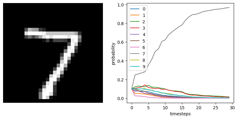
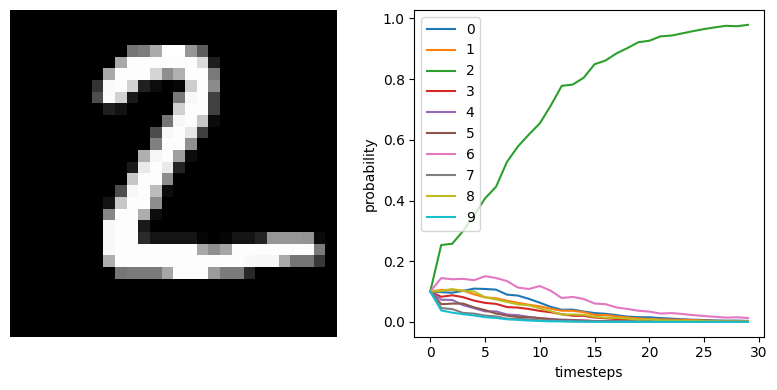
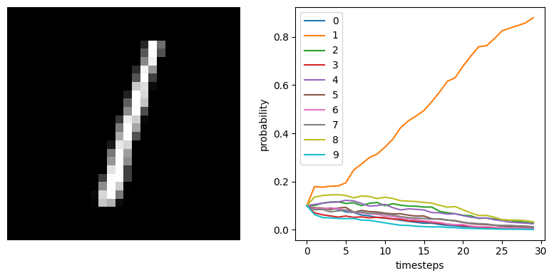
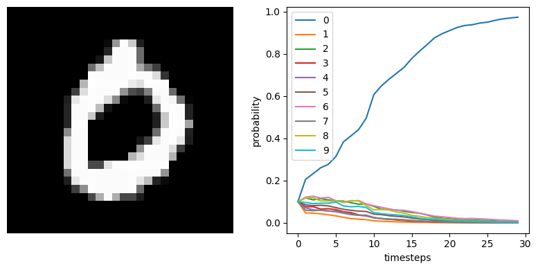
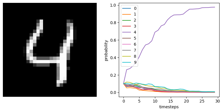
We can also plot some example outputs from the network, to see how it is performing over time.

data = sim.predict(test_images[:minibatch_size])

for i in range(5):
    plt.figure(figsize=(8, 4))
    plt.subplot(1, 2, 1)
    plt.imshow(test_images[i, 0].reshape((28, 28)), cmap="gray")
    plt.axis("off")

    plt.subplot(1, 2, 2)
    plt.plot(tf.nn.softmax(data[out_p_filt][i]))
    plt.legend([str(i) for i in range(10)], loc="upper left")
    plt.xlabel("timesteps")
    plt.ylabel("probability")
    plt.tight_layout()

1/1 [==============================] - 2s 2s/step

sim.close()