
- Introduction
- Installation
- User guide
- API reference
- Examples
- Coming from Nengo to NengoDL
- Coming from TensorFlow to NengoDL
- Integrating a Keras model into a Nengo network
- Optimizing a spiking neural network
- Converting a Keras model to a spiking neural network
- Legendre Memory Units in NengoDL
- Optimizing a cognitive model
- Optimizing a cognitive model with temporal dynamics
- Additional resources
- Project information
Integrating a Keras model into a Nengo network
Often we may want to define one part of our model in Nengo, and another part in TensorFlow. For example, suppose we are building a biological reinforcement learning model, but we’d like the inputs to our model to be natural images rather than artificial vectors. We could load a vision network from TensorFlow, insert it into our model using NengoDL, and then build the rest of our model using normal Nengo syntax.
NengoDL supports this through the TensorNode class. This allows us to write code directly in TensorFlow, and then insert it easily into Nengo. In this example we will demonstrate how to integrate a Keras network into a Nengo model in a series of stages. First, inserting an entire Keras model, second, inserting individual Keras layers, and third, using native Nengo objects.
[1]:
%matplotlib inline

import numpy as np
import matplotlib.pyplot as plt
import tensorflow as tf

import nengo
import nengo_dl

# keras uses the global random seeds, so we set those here to
# ensure the example is reproducible
seed = 0
np.random.seed(seed)
tf.random.set_seed(seed)
Introduction to TensorNodes
nengo_dl.TensorNode works very similarly to nengo.Node, except instead of using the node to insert Python code into our model we will use it to insert TensorFlow code.
The first thing we need to do is define our TensorNode output. This is a function that accepts the current simulation time (and, optionally, a batch of vectors) as input, and produces a batch of vectors as output. All of these variables will be represented as tf.Tensor objects, and the internal operations of the TensorNode will be implemented with TensorFlow operations. For example, we could use a TensorNode to output a sin function:
[2]:
with nengo.Network() as net:

    def sin_func(t):
        # compute sin wave (based on simulation time)
        output = tf.sin(t)

        # convert output to the expected batched vector shape
        # (with batch size of 1 and vector dimensionality 1)
        output = tf.reshape(output, (1, 1))

        return output

    node = nengo_dl.TensorNode(sin_func)
    p = nengo.Probe(node)

with nengo_dl.Simulator(net) as sim:
    sim.run(5.0)

plt.figure()
plt.plot(sim.trange(), sim.data[p])
plt.show()
Build finished in 0:00:00
Optimization finished in 0:00:00
Construction finished in 0:00:00
Simulation finished in 0:00:00
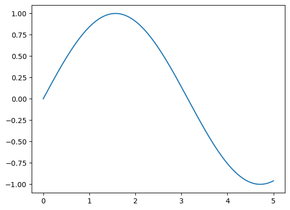
However, outputting a sin function is something we could do more easily with a regular nengo.Node. The main use case for nengo_dl.TensorNode is to allow us to write more complex TensorFlow code and insert it into a NengoDL model. For example, one thing we often want to do is take a deep network written in TensorFlow/Keras, and add it into a Nengo model, which is what we will focus on in this notebook.
Inserting a whole Keras model
Keras is a popular software package for building and training deep learning style networks. It is a higher-level API within TensorFlow to make it easier to construct and train deep networks. And because it is all implemented as a TensorFlow network under the hood, we can define a network using Keras and then insert it into NengoDL using a TensorNode.
This example assumes familiarity with the Keras API. Specifically it is based on the introduction in the Tensorflow documentation, so if you are not yet familiar with Keras, you may find it helpful to read those tutorials first.
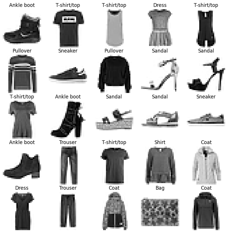
In this example we’ll train a neural network to classify the fashion MNIST dataset. This dataset contains images of clothing, and the goal of the network is to identify what type of clothing it is (e.g. t-shirt, trouser, coat, etc.).
[3]:
(train_images, train_labels), (
    test_images,
    test_labels,
) = tf.keras.datasets.fashion_mnist.load_data()

# normalize images so values are between 0 and 1
train_images = train_images / 255.0
test_images = test_images / 255.0

# flatten images
train_images = train_images.reshape((train_images.shape[0], -1))
test_images = test_images.reshape((test_images.shape[0], -1))

class_names = [
    "T-shirt/top",
    "Trouser",
    "Pullover",
    "Dress",
    "Coat",
    "Sandal",
    "Shirt",
    "Sneaker",
    "Bag",
    "Ankle boot",
]
num_classes = len(class_names)

plt.figure(figsize=(10, 10))
for i in range(25):
    plt.subplot(5, 5, i + 1)
    plt.imshow(train_images[i].reshape((28, 28)), cmap=plt.cm.binary)
    plt.axis("off")
    plt.title(class_names[train_labels[i]])
Next we build and train a simple neural network, using Keras. In this case we’re building a simple two layer, densely connected network.
Note that alternatively we could define the network in Keras and then train it in NengoDL (using the Simulator.fit function). But for now we’ll show how to do everything in Keras.
[4]:
inp = tf.keras.Input(train_images.shape[1:])
hidden = tf.keras.layers.Dense(units=128, activation=tf.nn.relu)(inp)
out = tf.keras.layers.Dense(units=num_classes)(hidden)

model = tf.keras.Model(inputs=inp, outputs=out)

model.compile(
    optimizer=tf.optimizers.Adam(),
    loss=tf.losses.SparseCategoricalCrossentropy(from_logits=True),
    metrics=["accuracy"],
)
model.fit(train_images, train_labels, epochs=5)

print("Test accuracy:", model.evaluate(test_images, test_labels, verbose=0)[1])
Epoch 1/5
1875/1875 [==============================] - 4s 2ms/step - loss: 0.4991 - accuracy: 0.8266
Epoch 2/5
1875/1875 [==============================] - 3s 2ms/step - loss: 0.3740 - accuracy: 0.8653
Epoch 3/5
1875/1875 [==============================] - 3s 2ms/step - loss: 0.3357 - accuracy: 0.8779
Epoch 4/5
1875/1875 [==============================] - 3s 2ms/step - loss: 0.3115 - accuracy: 0.8853
Epoch 5/5
1875/1875 [==============================] - 3s 2ms/step - loss: 0.2935 - accuracy: 0.8912
Test accuracy: 0.8691999912261963
We’ll save the trained weights, so that we can load them later within our TensorNode.
[5]:
model_weights = "keras_weights"
model.save_weights(model_weights)
Now we’re ready to create our TensorNode. Our TensorNode needs to be a bit more complicated in this case, since we need to load in the model from above and the pretrained weights. We can accomplish this by creating a custom Keras Layer, which allows us to define build and call methods.
We’ll use the build function to call the Keras clone_model function. This effectively reruns the Keras model definition from above, but because we’re calling it within the build stage it will be naturally integrated into the NengoDL model that is being built.
The call function is where we do the main job of constructing the TensorFlow elements that will implement our node. It will take TensorFlow Tensors as input and produce a tf.Tensor as output, as with the tf.sin example above. In this case we apply the Keras model to the TensorNode inputs. This adds the TensorFlow elements that implement that Keras model into the simulation graph.
[6]:
class KerasWrapper(tf.keras.layers.Layer):
    def __init__(self, keras_model):
        super().__init__()

        self.model = keras_model

    def build(self, input_shape):
        super().build(input_shape)

        # we use clone_model to re-build the model
        # within the TensorNode context
        self.model = tf.keras.models.clone_model(self.model)

        # load the weights we saved above
        self.model.load_weights(model_weights)

    def call(self, inputs):
        # apply the model to the inputs
        return self.model(inputs)
Now that we have our KerasWrapper class, we can use it to insert our Keras model into a Nengo network via a TensorNode. We simply instantiate a KerasWrapper (passing in our Keras model from above), and then pass that Layer object to the TensorNode.
[7]:
with nengo.Network() as net:
    # create a normal input node to feed in our test image.
    # the `np.ones` array is a placeholder, these
    # values will be replaced with the Fashion MNIST images
    # when we run the Simulator.
    input_node = nengo.Node(output=np.ones(28 * 28))

    # create an instance of the custom layer class we created,
    # passing it the Keras model
    layer = KerasWrapper(model)

    # create a TensorNode and pass it the new layer
    keras_node = nengo_dl.TensorNode(
        layer,
        shape_in=(28 * 28,),  # shape of input (the flattened images)
        shape_out=(num_classes,),  # shape of output (# of classes)
        pass_time=False,  # this node doesn't require time as input
    )

    # connect up our input to our keras node
    nengo.Connection(input_node, keras_node, synapse=None)

    # add a probe to collect output of keras node
    keras_p = nengo.Probe(keras_node)
At this point we could add any other Nengo components we like to the network, and connect them up to the Keras node (for example, if we wanted to take the classified image labels and use them as input to a spiking neural model). But to keep things simple, we’ll stop here.
Now we can evaluate the performance of the Nengo network, to see if we have successfully loaded the source Keras model.
[8]:
# unlike in Keras, NengoDl simulations always run over time.
# so we need to add the time dimension to our data (even though
# in this case we'll just run for a single timestep).
train_images = train_images[:, None, :]
train_labels = train_labels[:, None, None]

test_images = test_images[:, None, :]
test_labels = test_labels[:, None, None]
[9]:
with net:
    # we'll disable some features we don't need in this example, to improve
    # the training speed
    nengo_dl.configure_settings(stateful=False, use_loop=False)

minibatch_size = 20
with nengo_dl.Simulator(net, minibatch_size=minibatch_size) as sim:
    # call compile and evaluate, as we did with the Keras model
    sim.compile(
        loss=tf.losses.SparseCategoricalCrossentropy(from_logits=True),
        metrics=["accuracy"],
    )
    print(
        "Test accuracy:",
        sim.evaluate(test_images, test_labels, verbose=0)["probe_accuracy"],
    )
Build finished in 0:00:00
Optimization finished in 0:00:00
Construction finished in 0:00:00
Test accuracy: 0.8691999912261963
We can see that we’re getting the same performance in Nengo as we were in Keras, indicating that we have successfully inserted the Keras model into Nengo.
Inserting Keras layers
Rather than inserting an entire Keras model as a single block, we might want to integrate a Keras model into Nengo by inserting the individual layers. This requires more manual translation work, but it makes it easier to make changes to the model later on (for example, adding some spiking neuron layers).
We’ll keep everything the same as above (same data, same network structure), but this time we will recreate the Keras model one layer at a time.
As we saw above, we can wrap Keras Layers in a TensorNode by passing the layer object to the TensorNode. However, we can make this construction process even simpler by using nengo_dl.Layer. This is a different syntax for creating TensorNodes that mimics the Keras functional layer API. Under the hood it’s doing the same thing (creating TensorNodes and Connections), but it allows us to define the model in a way that looks very similar to the original Keras model definition.
[10]:
with nengo.Network(seed=seed) as net:
    # input node, same as before
    inp = nengo.Node(output=np.ones(28 * 28))

    # add the Dense layers, as in the Keras model
    hidden = nengo_dl.Layer(tf.keras.layers.Dense(units=128, activation=tf.nn.relu))(
        inp
    )
    out = nengo_dl.Layer(tf.keras.layers.Dense(units=num_classes))(hidden)

    # add a probe to collect output
    out_p = nengo.Probe(out)
Since we’re rebuilding the network within Nengo, we’ll need to train it within NengoDL this time. Fortunately, the API is essentially the same:
[11]:
with net:
    nengo_dl.configure_settings(stateful=False, use_loop=False)

with nengo_dl.Simulator(net, minibatch_size=minibatch_size) as sim:
    # call compile and fit with the same arguments as we used
    # in the original Keras model
    sim.compile(
        optimizer=tf.optimizers.Adam(),
        loss=tf.losses.SparseCategoricalCrossentropy(from_logits=True),
        metrics=["accuracy"],
    )
    sim.fit(train_images, train_labels, epochs=5)

    print(
        "Test accuracy:",
        sim.evaluate(test_images, test_labels, verbose=0)["probe_accuracy"],
    )
Build finished in 0:00:00
Optimization finished in 0:00:00
Construction finished in 0:00:00
Epoch 1/5
3000/3000 [==============================] - 6s 2ms/step - loss: 0.4857 - probe_loss: 0.4857 - probe_accuracy: 0.8283
Epoch 2/5
3000/3000 [==============================] - 6s 2ms/step - loss: 0.3672 - probe_loss: 0.3672 - probe_accuracy: 0.8669
Epoch 3/5
3000/3000 [==============================] - 5s 2ms/step - loss: 0.3333 - probe_loss: 0.3333 - probe_accuracy: 0.8783
Epoch 4/5
3000/3000 [==============================] - 6s 2ms/step - loss: 0.3093 - probe_loss: 0.3093 - probe_accuracy: 0.8866
Epoch 5/5
3000/3000 [==============================] - 6s 2ms/step - loss: 0.2919 - probe_loss: 0.2919 - probe_accuracy: 0.8922
Test accuracy: 0.8781999945640564
We can see that we’re getting basically the same performance as before (with minor differences due to a different random initialization).
Building an equivalent network with Nengo objects
In the above examples we used TensorNodes to insert TensorFlow code into Nengo, starting with a whole model and then with individual layers. The next thing we might want to do is directly define an equivalent network using native Nengo objects, rather than doing everything through TensorNodes. One advantage of this approach is that a native Nengo network will be able to run on any Nengo-supported platform (e.g., custom neuromorphic hardware), whereas TensorNodes will only work within NengoDL.
We can create the same network structure (two densely connected layers), by using nengo.Ensemble and nengo.Connection:
[12]:
with nengo.Network(seed=seed) as net:
    # set up some default parameters to match the Keras defaults
    net.config[nengo.Ensemble].gain = nengo.dists.Choice([1])
    net.config[nengo.Ensemble].bias = nengo.dists.Choice([0])
    net.config[nengo.Connection].synapse = None
    net.config[nengo.Connection].transform = nengo_dl.dists.Glorot()

    # input node, same as before
    inp = nengo.Node(output=np.ones(28 * 28))

    # add the first dense layer
    hidden = nengo.Ensemble(128, 1, neuron_type=nengo.RectifiedLinear()).neurons
    nengo.Connection(inp, hidden)

    # add the linear output layer (using nengo.Node since there is
    # no nonlinearity)
    out = nengo.Node(size_in=num_classes)
    nengo.Connection(hidden, out)

    # add a probe to collect output
    out_p = nengo.Probe(out)
And then the training works exactly the same as before:
[13]:
with net:
    nengo_dl.configure_settings(stateful=False, use_loop=False)

with nengo_dl.Simulator(net, minibatch_size=minibatch_size) as sim:
    sim.compile(
        optimizer=tf.optimizers.Adam(),
        loss=tf.losses.SparseCategoricalCrossentropy(from_logits=True),
        metrics=["accuracy"],
    )
    sim.fit(train_images, train_labels, epochs=5)

    print(
        "Test accuracy:",
        sim.evaluate(test_images, test_labels, verbose=0)["probe_accuracy"],
    )
Build finished in 0:00:00
Optimization finished in 0:00:00
Construction finished in 0:00:00
Epoch 1/5
3000/3000 [==============================] - 6s 2ms/step - loss: 0.4898 - probe_loss: 0.4898 - probe_accuracy: 0.8283
Epoch 2/5
3000/3000 [==============================] - 6s 2ms/step - loss: 0.3699 - probe_loss: 0.3699 - probe_accuracy: 0.8653
Epoch 3/5
3000/3000 [==============================] - 6s 2ms/step - loss: 0.3365 - probe_loss: 0.3365 - probe_accuracy: 0.8770
Epoch 4/5
3000/3000 [==============================] - 6s 2ms/step - loss: 0.3130 - probe_loss: 0.3130 - probe_accuracy: 0.8841
Epoch 5/5
3000/3000 [==============================] - 6s 2ms/step - loss: 0.2943 - probe_loss: 0.2943 - probe_accuracy: 0.8917
Test accuracy: 0.8780999779701233
Again we can see that we’re getting roughly the same accuracy as before.
We could also use the nengo_dl.Converter tool to automatically perform this translation from Keras to native Nengo objects. Under the hood this is doing the same thing as we did above (creating Nodes, Ensembles, Connections, and Probes), but nengo_dl.Converter removes some of the manual effort in that translation process.
[14]:
converter = nengo_dl.Converter(model)

with converter.net:
    nengo_dl.configure_settings(stateful=False, use_loop=False)

with nengo_dl.Simulator(converter.net, minibatch_size=minibatch_size) as sim:
    # the Converter will copy the parameters from the Keras model, so we don't
    # need to do any further training (although we could if we wanted)
    sim.compile(
        loss=tf.losses.SparseCategoricalCrossentropy(from_logits=True),
        metrics=["accuracy"],
    )

    print(
        "Test accuracy:",
        sim.evaluate(test_images, test_labels, verbose=0)["probe_accuracy"],
    )
Build finished in 0:00:00
Optimization finished in 0:00:00
Construction finished in 0:00:00
Constructing graph: build stage finished in 0:00:00
/home/travis-ci/tmp/nengo-dl-4136466773-1/nengo-dl/nengo_dl/simulator.py:1736: UserWarning: Number of elements (1) in ['ndarray'] does not match number of Nodes (2); consider using an explicit input dictionary in this case, so that the assignment of data to objects is unambiguous.
  warnings.warn(
Test accuracy: 0.8691999912261963
Note that in this case the performance of the Nengo network exactly matches the original Keras model, since the Converter copied over the parameter values. See the documentation for more details on using nengo_dl.Converter.
Conclusion
We have seen three different methods for integrating a Keras model into NengoDL: inserting a whole model, inserting individual layers, or building an equivalent native Nengo model. Each method reproduces the same behaviour as the original Keras model, but requires differing levels of effort and supports different functionality. The most appropriate method will depend on your use case, but here are some rough guidelines.
Inserting a whole model
The main advantage of this approach is that we can use exactly the same model definition. The disadvantage is that the model is essentially still just a Keras model, so it won’t be able to incorporate any of the unique features of NengoDL (like spiking neurons). But if you just need to add a standard deep network into your Nengo model, then this is probably the way to go!
Inserting individual layers
This approach strikes a balance: we can still use the familiar Keras Layer syntax, but we have increased flexibility to modify the network architecture. If inserting a whole model doesn’t meet your needs, but you don’t care about running your model in any Nengo frameworks other than NengoDL, then try this method.
Building a native Nengo model
This approach requires the most modification of the original model, as it requires us to translate Keras syntax into Nengo syntax. However, by building a native Nengo model we gain the full advantages of the Nengo framework, such as cross-platform compatibility. That allows us to do things like train a network in NengoDL and then run it on custom neuromorphic hardware. And we can use the nengo_dl.Converter tool to automate this translation process. If neither of the above approaches are
meeting your needs, then dive fully into Nengo!