Converting a Keras model to an SNN on Loihi

This notebook describes how to train a network in Keras and convert it to a spiking neural network (SNN) to run on Loihi. Intel’s Loihi chip is a type of “neuromorphic” hardware—specialized neural network acceleration hardware that uses spike-based communication like neurons in the brain. In this tutorial, will look at how to set up our network to target and run on Intel’s Loihi chip using the NengoLoihi backend. While in general the Nengo ecosystem allows users to switch between backends without changes to their models, we will see how making some Loihi-specific changes during training and inference allow us to take full advantage of its capabilities.

There are several ways to build SNNs to target NengoLoihi. The CIFAR-10 Loihi example works through how to build up a deep spiking network to run on Loihi using the standard Nengo and NengoDL APIs. In NengoDL’s Keras to SNN example, we looked at converting a Keras model to an SNN. Here, we will extend the Keras to SNN example, tailoring the model for execution on Loihi.

The goal of this notebook is to familiarize you with some of the nuances of running SNNs on the Loihi, and how to set these up starting from a neural network defined in Keras. The two focuses in this notebook are on adding a network layer that runs off-chip to transform the input images into spikes, and training using a Loihi neuron model that captures the unique behaviour of Loihi’s quantized neurons. We’ll add the network layer and train and test with normal ReLU neurons first to see what kind of performance we can expect without quantization constraints. Then we’ll train with the Loihi neurons to improve implementation performance, and finally we’ll run the model on Loihi to measure the final performance (we use a simulated Loihi if actual Loihi hardware is not available).

import collections
import warnings

%matplotlib inline
import matplotlib.pyplot as plt
import nengo
import nengo_dl
import numpy as np
import tensorflow as tf

import nengo_loihi

# ignore NengoDL warning about no GPU
warnings.filterwarnings("ignore", message="No GPU", module="nengo_dl")

# The results in this notebook should be reproducible across many random seeds.
# However, some seed values may cause problems, particularly in the `to-spikes` layer
# where poor initialization can result in no information being sent to the chip. We set
# the seed to ensure that good results are reproducible without having to re-train.
np.random.seed(0)
tf.random.set_seed(0)

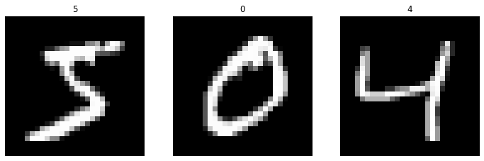
In this example we’ll use the standard MNIST dataset.

# load in MNIST dataset
(
    (train_images, train_labels),
    (test_images, test_labels),
) = tf.keras.datasets.mnist.load_data()

# flatten images and add time dimension
train_images = train_images.reshape((train_images.shape[0], 1, -1))
train_labels = train_labels.reshape((train_labels.shape[0], 1, -1))
test_images = test_images.reshape((test_images.shape[0], 1, -1))
test_labels = test_labels.reshape((test_labels.shape[0], 1, -1))

plt.figure(figsize=(12, 4))
for i in range(3):
    plt.subplot(1, 3, i + 1)
    plt.imshow(np.reshape(train_images[i], (28, 28)), cmap="gray")
    plt.axis("off")
    plt.title(str(train_labels[i, 0, 0]))

Implementing the network

We will start with the same network structure used in the Keras to SNN example: Two convolutional layers and a dense layer.

The only way to communicate with the Loihi is by sending spikes. Usually, when we have a model that we want to run on neuromorphic hardware, we want the whole model that we’ve defined to run on the hardware. Communicating with Loihi, however, requires that we have at least one layer that runs off-chip to convert the input signal to spikes to send to the rest of the model running on Loihi.

We’ll add a Conv2D layer to run off-chip and convert the input signal to spikes. This could also be an Activation layer. The advantage to the Activation layer is that it adds no extra parameters and minimizes off-chip computations. The Conv2D layer uses a few parameters, and requires a bit more off-chip computation, but gives the network much more flexibility as to how pixels are converted to spikes. An Activation layer would likely work well for simple images like MNIST, but for more complex images (e.g. with more than one color channel, or a wider range of intensity values) the flexibility of the Conv2D layer is important. We avoid layers like the Dense layer, as it significantly increases both the number of parameters and the number of computations that have to be run off-chip.

On the output side of the network, we now have to worry about how many neurons are in the last layer run on the chip. We are limited in how many neurons we can record from on the board, so we add a Dense layer with 100 neurons between the last Conv2D layer and our 10-dimensional Dense output layer (which runs off-chip). This way, we only have to record from 100 neurons, rather than the 2,304 neurons we would need to record from if we connected directly from the last Conv2D layer to the 10-dimensional output. An added benefit is that the amount of off-chip computation is reduced, since the number of weights used by the off-chip output layer is 100 x 10 instead of 2304 x 10.

inp = tf.keras.Input(shape=(28, 28, 1), name="input")

# transform input signal to spikes using trainable 1x1 convolutional layer
to_spikes_layer = tf.keras.layers.Conv2D(
    filters=3,  # 3 neurons per pixel
    kernel_size=1,
    strides=1,
    activation=tf.nn.relu,
    use_bias=False,
    name="to-spikes",
)
to_spikes = to_spikes_layer(inp)

# on-chip convolutional layers
conv0_layer = tf.keras.layers.Conv2D(
    filters=32,
    kernel_size=3,
    strides=2,
    activation=tf.nn.relu,
    use_bias=False,
    name="conv0",
)
conv0 = conv0_layer(to_spikes)

conv1_layer = tf.keras.layers.Conv2D(
    filters=64,
    kernel_size=3,
    strides=2,
    activation=tf.nn.relu,
    use_bias=False,
    name="conv1",
)
conv1 = conv1_layer(conv0)

flatten = tf.keras.layers.Flatten(name="flatten")(conv1)

dense0_layer = tf.keras.layers.Dense(units=100, activation=tf.nn.relu, name="dense0")
dense0 = dense0_layer(flatten)

# since this final output layer has no activation function,
# it will be converted to a `nengo.Node` and run off-chip
dense1 = tf.keras.layers.Dense(units=10, name="dense1")(dense0)

model = tf.keras.Model(inputs=inp, outputs=dense1)
model.summary()

Model: "model"
_________________________________________________________________
Layer (type)                 Output Shape              Param #
=================================================================
input (InputLayer)           [(None, 28, 28, 1)]       0
_________________________________________________________________
to-spikes (Conv2D)           (None, 28, 28, 3)         3
_________________________________________________________________
conv0 (Conv2D)               (None, 13, 13, 32)        864
_________________________________________________________________
conv1 (Conv2D)               (None, 6, 6, 64)          18432
_________________________________________________________________
flatten (Flatten)            (None, 2304)              0
_________________________________________________________________
dense0 (Dense)               (None, 100)               230500
_________________________________________________________________
dense1 (Dense)               (None, 10)                1010
=================================================================
Total params: 250,809
Trainable params: 250,809
Non-trainable params: 0
_________________________________________________________________

2022-01-21 13:06:06.315597: W tensorflow/core/common_runtime/gpu/gpu_bfc_allocator.cc:39] Overriding allow_growth setting because the TF_FORCE_GPU_ALLOW_GROWTH environment variable is set. Original config value was 0.

Training the networks

As in the Keras-to-SNN notebook, once we create our model we’ll use the NengoDL Converter to translate it into a Nengo network, and then we’ll train.

def train(params_file="./keras_to_loihi_params", epochs=1, **kwargs):
    converter = nengo_dl.Converter(model, **kwargs)

    with nengo_dl.Simulator(converter.net, seed=0, minibatch_size=200) as sim:
        sim.compile(
            optimizer=tf.optimizers.RMSprop(0.001),
            loss={
                converter.outputs[dense1]: tf.losses.SparseCategoricalCrossentropy(
                    from_logits=True
                )
            },
            metrics={converter.outputs[dense1]: tf.metrics.sparse_categorical_accuracy},
        )
        sim.fit(
            {converter.inputs[inp]: train_images},
            {converter.outputs[dense1]: train_labels},
            epochs=epochs,
        )

        # save the parameters to file
        sim.save_params(params_file)

# train this network with normal ReLU neurons
train(
    epochs=2,
    swap_activations={tf.nn.relu: nengo.RectifiedLinear()},
)

Build finished in 0:00:00
Optimization finished in 0:00:00
Construction finished in 0:00:00
Epoch 1/2
Constructing graph: build stage finished in 0:00:00

2022-01-21 13:06:09.301844: W tensorflow/stream_executor/gpu/asm_compiler.cc:77] Couldn't get ptxas version string: Internal: Couldn't invoke ptxas --version
2022-01-21 13:06:09.302516: W tensorflow/stream_executor/gpu/redzone_allocator.cc:314] Internal: Failed to launch ptxas
Relying on driver to perform ptx compilation.
Modify $PATH to customize ptxas location.
This message will be only logged once.

300/300 [==============================] - 6s 10ms/step - loss: 0.1796 - probe_loss: 0.1796 - probe_sparse_categorical_accuracy: 0.9461
Epoch 2/2
300/300 [==============================] - 3s 10ms/step - loss: 0.0486 - probe_loss: 0.0486 - probe_sparse_categorical_accuracy: 0.9852

After training for 2 epochs the non-spiking network achievs around 98% accuracy on the test data.

Now that we have our trained weights, we can begin the conversion to spiking neurons. To help us in this process we’re going to first define a helper function that will build the network for us, load weights from a specified file, and make it easy to play around with some other features of the network.

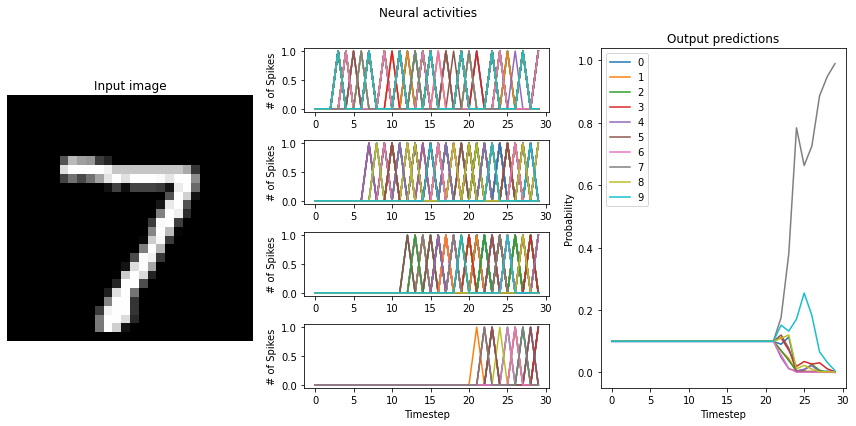
Evaluating the networks

We will now define a general function to evaluate our network on the test dataset with various neural activation functions (both non-spiking and spiking). The function creates a new network with the desired activation function, loads the weights that we learned during training, runs the network on the test dataset, and reports accuracy and firing rate with both print statements and plots.

def run_network(
    activation,
    params_file="./keras_to_loihi_params",
    n_steps=30,
    scale_firing_rates=1,
    synapse=None,
    n_test=100,
    n_plots=2,
):
    # convert the keras model to a nengo network
    nengo_converter = nengo_dl.Converter(
        model,
        scale_firing_rates=scale_firing_rates,
        swap_activations={tf.nn.relu: activation},
        synapse=synapse,
    )

    # get input/output objects
    nengo_input = nengo_converter.inputs[inp]
    nengo_output = nengo_converter.outputs[dense1]

    # add probes to layers to record activity
    with nengo_converter.net:
        probes = collections.OrderedDict(
            [
                [to_spikes_layer, nengo.Probe(nengo_converter.layers[to_spikes])],
                [conv0_layer, nengo.Probe(nengo_converter.layers[conv0])],
                [conv1_layer, nengo.Probe(nengo_converter.layers[conv1])],
                [dense0_layer, nengo.Probe(nengo_converter.layers[dense0])],
            ]
        )

    # repeat inputs for some number of timesteps
    tiled_test_images = np.tile(test_images[:n_test], (1, n_steps, 1))

    # set some options to speed up simulation
    with nengo_converter.net:
        nengo_dl.configure_settings(stateful=False)

    # build network, load in trained weights, run inference on test images
    with nengo_dl.Simulator(
        nengo_converter.net, minibatch_size=20, progress_bar=False
    ) as nengo_sim:
        nengo_sim.load_params(params_file)
        data = nengo_sim.predict({nengo_input: tiled_test_images})

    # compute accuracy on test data, using output of network on
    # last timestep
    test_predictions = np.argmax(data[nengo_output][:, -1], axis=-1)
    print(
        "Test accuracy: %.2f%%"
        % (100 * np.mean(test_predictions == test_labels[:n_test, 0, 0]))
    )

    # plot the results
    mean_rates = []
    for i in range(n_plots):
        plt.figure(figsize=(12, 6))

        plt.subplot(1, 3, 1)
        plt.title("Input image")
        plt.imshow(test_images[i, 0].reshape((28, 28)), cmap="gray")
        plt.axis("off")

        n_layers = len(probes)
        mean_rates_i = []
        for j, layer in enumerate(probes.keys()):
            probe = probes[layer]
            plt.subplot(n_layers, 3, (j * 3) + 2)
            plt.suptitle("Neural activities")

            outputs = data[probe][i]

            # look at only at non-zero outputs
            nonzero = (outputs > 0).any(axis=0)
            outputs = outputs[:, nonzero] if sum(nonzero) > 0 else outputs

            # undo neuron amplitude to get real firing rates
            outputs /= nengo_converter.layers[layer].ensemble.neuron_type.amplitude

            rates = outputs.mean(axis=0)
            mean_rate = rates.mean()
            mean_rates_i.append(mean_rate)
            print(
                '"%s" mean firing rate (example %d): %0.1f' % (layer.name, i, mean_rate)
            )

            if is_spiking_type(activation):
                outputs *= 0.001
                plt.ylabel("# of Spikes")
            else:
                plt.ylabel("Firing rates (Hz)")

            # plot outputs of first 100 neurons
            plt.plot(outputs[:, :100])

        mean_rates.append(mean_rates_i)

        plt.xlabel("Timestep")

        plt.subplot(1, 3, 3)
        plt.title("Output predictions")
        plt.plot(tf.nn.softmax(data[nengo_output][i]))
        plt.legend([str(j) for j in range(10)], loc="upper left")
        plt.xlabel("Timestep")
        plt.ylabel("Probability")

        plt.tight_layout()

    # take mean rates across all plotted examples
    mean_rates = np.array(mean_rates).mean(axis=0)

    return mean_rates


def is_spiking_type(neuron_type):
    return isinstance(neuron_type, (nengo.LIF, nengo.SpikingRectifiedLinear))

# test the trained networks on test set
mean_rates = run_network(activation=nengo.RectifiedLinear(), n_steps=10)

Test accuracy: 100.00%
"to-spikes" mean firing rate (example 0): 14.2
"conv0" mean firing rate (example 0): 2.0
"conv1" mean firing rate (example 0): 1.0
"dense0" mean firing rate (example 0): 2.8
"to-spikes" mean firing rate (example 1): 15.6
"conv0" mean firing rate (example 1): 2.3
"conv1" mean firing rate (example 1): 1.4
"dense0" mean firing rate (example 1): 3.7

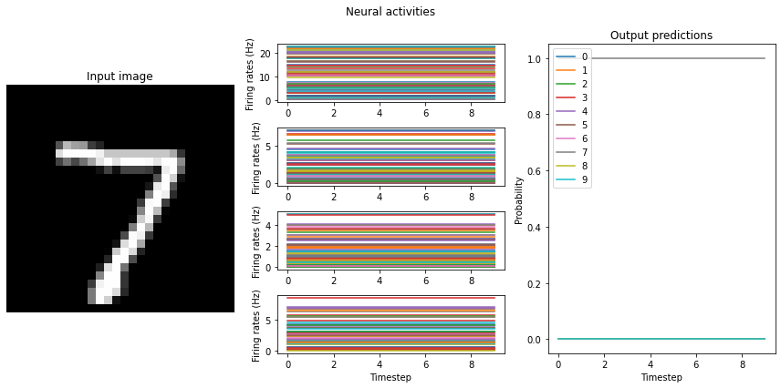
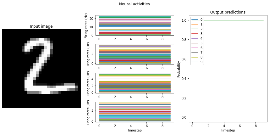
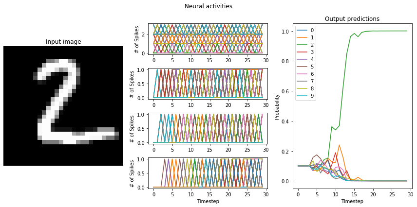
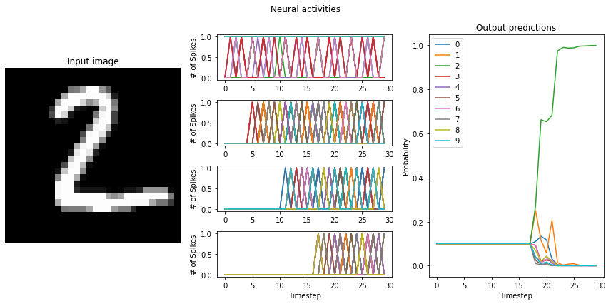
Note that we’re plotting the output over time for consistency with future plots, but since our network doesn’t have any temporal elements (e.g. spiking neurons), the output is constant for each digit. The firing rates here displayed in the middle graph are important to note for conversion to spikes, and may vary somewhat depending on the random initial conditions used for training. One of the important features visible here, which we’ll discuss shortly, is the decreasing mean firing rate as you move through the network. Note that these mean firing rates are computed across only the neurons that have non-zero activities; they are therefore the mean rates of the active neurons.

Let’s continue with the comparison by moving into spikes.

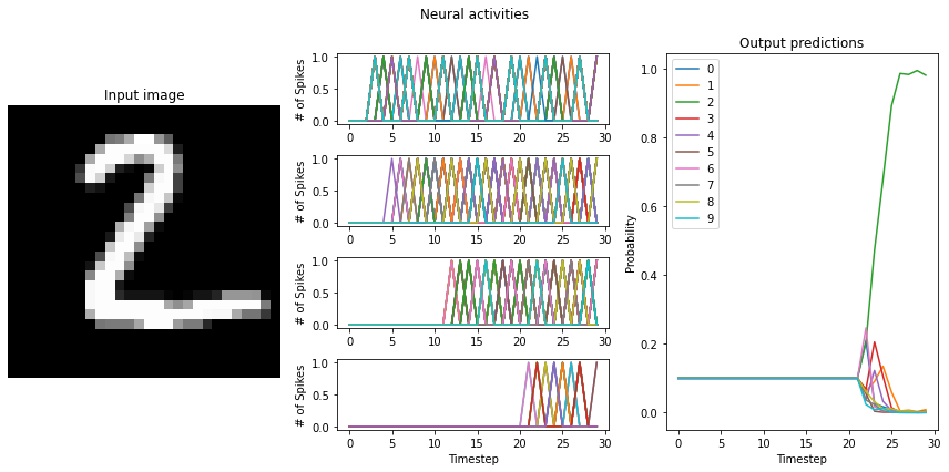
Converting to a spiking neural network

Using the NengoDL converter, we can swap all the relu activation functions to nengo.SpikingRectifiedLinear. Using the lessons that we learned in the Keras->SNN example notebook we’ll set synapse=0.005 and scale_firing_rates=100.

# test the trained networks using spiking neurons
run_network(
    activation=nengo.SpikingRectifiedLinear(),
    scale_firing_rates=100,
    synapse=0.005,
)

Test accuracy: 100.00%
"to-spikes" mean firing rate (example 0): 1434.5
"conv0" mean firing rate (example 0): 184.6
"conv1" mean firing rate (example 0): 88.6
"dense0" mean firing rate (example 0): 143.2
"to-spikes" mean firing rate (example 1): 1561.8
"conv0" mean firing rate (example 1): 210.9
"conv1" mean firing rate (example 1): 98.7
"dense0" mean firing rate (example 1): 192.1

array([1498.1554 ,  197.74052,   93.66748,  167.63669], dtype=float32)

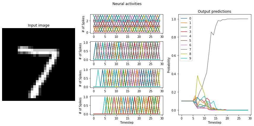
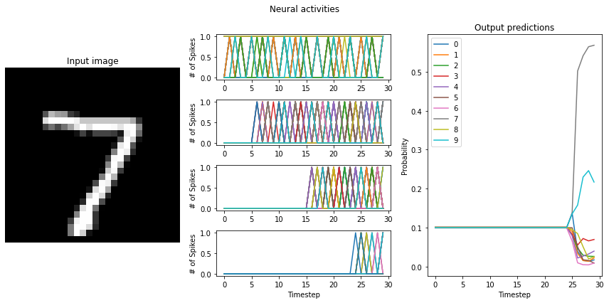
An important feature of SNNs is the time required to generate output. The larger your scaling factor, the quicker the network response to input will be. This is because more spikes will be generated at each layer, triggering a quicker response at the succeeding layer.

For still images, where each successive image has no correlation with the previous image, this leads to a lag in generating output. SNNs are however much more efficient in a problem like processing a video stream, where there is high correlation between frames. In general, SNNs perform better in situations with temporal dynamics. For simplicity, though, we only examine the case of processing still images here.

Let’s see what happens when we convert to an SNN using Loihi neurons.

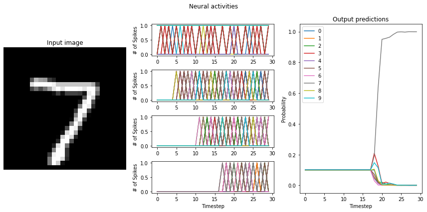
Converting to SNN using Loihi neurons

To get a sense of how well our network will run on Loihi, we switch to using the LoihiSpikingRectifiedLinear activation profile.

Note that the on-chip restrictions don’t apply to the input layer that we added to the network, because it won’t be running on the Loihi. Here, the performance differences are minimal so we just convert all neurons over to Loihi neurons. If you find that adding the input layer is causing a performance drop, you may want to build your network such that only the on-chip layers use the NengoLoihi neurons and the off-chip layer uses a standard spiking neuron model (i.e. SpikingRectifiedLinear).

# test the trained networks using spiking neurons
run_network(
    activation=nengo_loihi.neurons.LoihiSpikingRectifiedLinear(),
    scale_firing_rates=100,
    synapse=0.005,
)

Test accuracy: 89.00%
"to-spikes" mean firing rate (example 0): 792.1
"conv0" mean firing rate (example 0): 92.8
"conv1" mean firing rate (example 0): 47.5
"dense0" mean firing rate (example 0): 36.5
"to-spikes" mean firing rate (example 1): 834.5
"conv0" mean firing rate (example 1): 102.7
"conv1" mean firing rate (example 1): 48.8
"dense0" mean firing rate (example 1): 38.1

array([813.3253  ,  97.74296 ,  48.18663 ,  37.301582], dtype=float32)

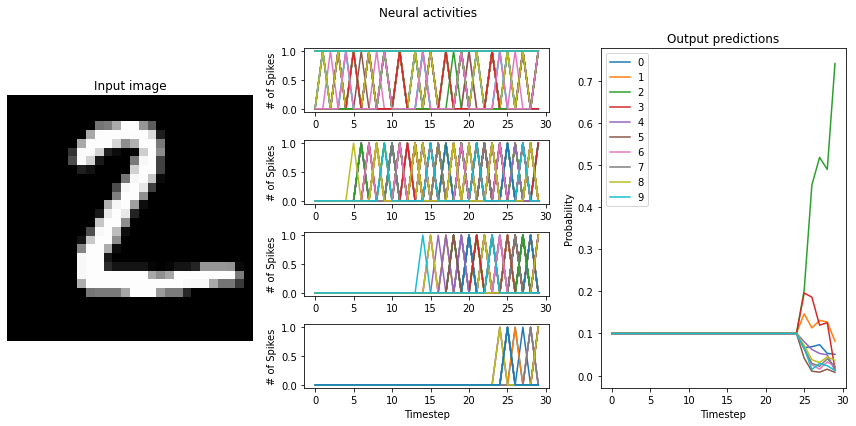
If the training resulted a network with large differences between the firing rates (> 10Hz) of the network layers, switching to LoihiSpikingRectifiedLinear neurons will cause a significant decrease in the performance of the network. What causes this?

Basically, the issue is that each of the layers need different scaling terms. With large firing rate discrepancies between layers, we end up trying to balance between having a scale_firing_rate value for the network that 1) is high enough to achieve good performance from the network, but 2) is low enough to not induce multiple spikes per time step in any layer. The second point here is where we’re getting tripped up.

Loihi neurons can only spike once per time step. Recall that while the scale_firing_rates term increases the gain on signals going into neurons, it also correspondingly decreases the amplitude of the neuron activity output. If scale_firing_rates is set high enough to expect three spikes per time step, but only one spike comes out, the effects will no longer balance out and performance will deteriorate.

Instead of setting a single scale_firing_rate for the whole network, we can specify a scaling value for each layer. To figure out what range we want to put the firing rates into, let’s look at the Loihi neurons’ activation functions.

The Loihi activation profile

The shape of the Loihi neuron activation profile is unique, and for high firing rates has strong discrepancies with standard relu and lif behaviour. This is due to the discretization required by the Loihi hardware. Let’s take a closer look.

def plot_activation(neurons, min, max, **kwargs):
    x = np.arange(min, max, 0.001)
    fr = neurons.rates(x=x, gain=[1], bias=[0])

    plt.plot(x, fr, lw=2, **kwargs)
    plt.title("%s with [gain=1, bias=0]" % str(neurons))
    plt.ylabel("Firing rate (Hz)")
    plt.xlabel("Input signal")
    plt.legend(["Standard", "Loihi"], loc=2)


plt.figure(figsize=(10, 3))
plot_activation(nengo.RectifiedLinear(), -100, 1000)
plot_activation(nengo_loihi.neurons.LoihiSpikingRectifiedLinear(), -100, 1000)

plt.figure(figsize=(10, 3))
plot_activation(nengo.LIF(), -4, 40)
plot_activation(nengo_loihi.neurons.LoihiLIF(), -4, 40)

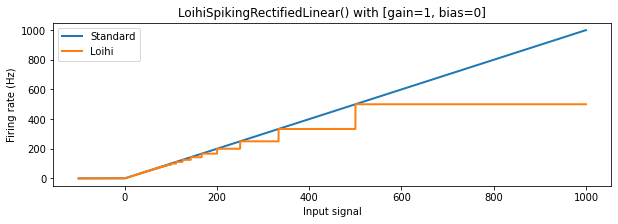
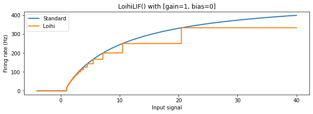
We can see that for lower firing rates the behaviour of the Loihi neurons approximates the normal relu and lif neurons relatively well, but for higher firing rates the discrepancy becomes larger. The discretization results in large plateus of input signal values where the output firing rate from the neuron stays the same, making different input values in this range indistinguishable. Also, as mentioned above, for input values above 1000 (not shown) the LoihiSpikingRectifiedLinear neuron will have a constant output of 1000 Hz (since this corresponds to one spike per timestep, the maximum firing rate on Loihi); the SpikingRectifiedLinear neuron, on the other hand, is able to fire faster than 1000 Hz by using multiple spikes per timestep.

We can now return to our original question: How do we pick good firing rates for each layer? For outputs above 250 Hz, both Loihi activation functions show significant deviations from the non-Loihi activation profiles; they also become more discontinuous above this point. We therefore want to keep our maximum firing rates below 250 Hz. We also need the firing rate to be high enough to generate sufficient spikes, so that information can be transmitted from layer to layer in a reasonable time. For these reasons, we’ll choose a target mean firing rate for each layer to be 200. We’ll generate a scaling term for each layer individually to hit this target.

target_mean = 200
scale_firing_rates = {
    to_spikes_layer: target_mean / mean_rates[0],
    conv0_layer: target_mean / mean_rates[1],
    conv1_layer: target_mean / mean_rates[2],
    dense0_layer: target_mean / mean_rates[3],
}

# test the trained networks using spiking neurons
run_network(
    activation=nengo_loihi.neurons.LoihiSpikingRectifiedLinear(),
    scale_firing_rates=scale_firing_rates,
    synapse=0.005,
)

Test accuracy: 98.00%
"to-spikes" mean firing rate (example 0): 169.2
"conv0" mean firing rate (example 0): 123.1
"conv1" mean firing rate (example 0): 93.0
"dense0" mean firing rate (example 0): 44.0
"to-spikes" mean firing rate (example 1): 191.0
"conv0" mean firing rate (example 1): 138.5
"conv1" mean firing rate (example 1): 98.6
"dense0" mean firing rate (example 1): 45.3

array([180.12039 , 130.82814 ,  95.81003 ,  44.690475], dtype=float32)

As we can see, when we individually scale the activity of each layer, we almost fully recover non-spiking performance. Note that the firing rates of some layers (the later layers in particular) do not quite meet the target mean firing rate of 200 Hz, though. This is because our mean firing rates were measured using the RectifiedLinear neuron type, and do not account for the difference between it and the LoihiSpikingRectifiedLinear activation function. For better results, we could go back and measure the mean firing rates using the Loihi neuron type, or hand-tune the scaling factors on each layer to achieve the desired firing rates.

Alternatively, we can train our network using the LoihiSpikingRectifiedLinear. This will account both for the discretization in the activation profile, and the hard limit of 1 spike per time step. For larger or more complex networks this can save time tuning.

Training with the Loihi neurons

We’re going to use another trick for training and set scale_firing_rates=100 while training. What this does essentially is initiate the network with high firing rates, such that during training we’ll consistently find a local minima with higher firing rates that will work well when we swap in spiking neurons. It also reduces the discrepancy in firing rates between layers, starting them all off in a higher range.

This is a low-overhead, ad-hoc means of increasing the firing rates of neurons in each layer, and does not guarantee that the network converges to a desired range of firing rates for each layer after training. The firing rate regularization method—shown in a basic form in the Keras to SNN example and in a more powerful form in the CIFAR-10 Loihi example—is a more consistent way to achieve the desired range of firing rates in each layer.

# train this network with normal ReLU neurons
train(
    params_file="./keras_to_loihi_loihineuron_params",
    epochs=2,
    swap_activations={tf.nn.relu: nengo_loihi.neurons.LoihiSpikingRectifiedLinear()},
    scale_firing_rates=100,
)

Build finished in 0:00:00
Optimization finished in 0:00:00
Construction finished in 0:00:00
Epoch 1/2
300/300 [==============================] - 6s 14ms/step - loss: 0.1944 - probe_loss: 0.1944 - probe_sparse_categorical_accuracy: 0.9392
Epoch 2/2
300/300 [==============================] - 4s 15ms/step - loss: 0.0613 - probe_loss: 0.0613 - probe_sparse_categorical_accuracy: 0.9807

Now when we run the network we need to be sure to again set the scale_firing_rates parameter so that the training conditions are replicated.

# test the trained networks using spiking neurons
run_network(
    activation=nengo_loihi.neurons.LoihiSpikingRectifiedLinear(),
    scale_firing_rates=100,
    params_file="./keras_to_loihi_loihineuron_params",
    synapse=0.005,
)

Test accuracy: 99.00%
"to-spikes" mean firing rate (example 0): 869.9
"conv0" mean firing rate (example 0): 131.5
"conv1" mean firing rate (example 0): 84.2
"dense0" mean firing rate (example 0): 107.9
"to-spikes" mean firing rate (example 1): 874.7
"conv0" mean firing rate (example 1): 138.4
"conv1" mean firing rate (example 1): 85.2
"dense0" mean firing rate (example 1): 112.8

array([872.3013  , 134.93323 ,  84.713806, 110.35761 ], dtype=float32)

This is another way that we can recover normal ReLU performance using Loihi neurons.

As discussed in the Keras to SNN example, we can also train up this network using an extra term added to the loss function as a way of getting neurons into the desired range of firing rates. This method has the benefit of being more precise in the resultant firing rates of neurons in the network. When we set scale_firing_rates to a large number during training, we’re simply instantiating the network with high firing rates and hoping it converges while maintaining these higher firing rates, but there is no guarantee. Adding the rate regularization term to the loss function ensures that the firing rates stay near their targets throughout the training process.

Running your SNN on Loihi

At this point we’re ready to test out our network on the Loihi. To actually run it on Loihi we have to set up a few more configuration parameters.

We’ll start by converting our network same as before, using the same parameters on the Converter call:

pres_time = 0.03  # how long to present each input, in seconds
n_test = 5  # how many images to test

# convert the keras model to a nengo network
nengo_converter = nengo_dl.Converter(
    model,
    scale_firing_rates=400,
    swap_activations={tf.nn.relu: nengo_loihi.neurons.LoihiSpikingRectifiedLinear()},
    synapse=0.005,
)
net = nengo_converter.net

# get input/output objects
nengo_input = nengo_converter.inputs[inp]
nengo_output = nengo_converter.outputs[dense1]

The next thing we need to do is load in the trained parameters. This involves creating a NengoDL Simulator, loading in the weights, and then calling the `freeze_params <https://www.nengo.ai/nengo-dl/reference.html#nengo_dl.Simulator.freeze_params>`__ function to save the weights to the network object. This will then let us build a network with the trained weights inside the NengoLoihi Simulator.

# build network, load in trained weights, save to network
with nengo_dl.Simulator(net) as nengo_sim:
    nengo_sim.load_params("keras_to_loihi_loihineuron_params")
    nengo_sim.freeze_params(net)

Build finished in 0:00:00
Optimization finished in 0:00:00
Construction finished in 0:00:00

Before we build the network in NengoLoihi we need to make a few more changes.

The input Node needs to altered to generate our test images as output:

with net:
    nengo_input.output = nengo.processes.PresentInput(
        test_images, presentation_time=pres_time
    )

We specify that the to_spikes layer should run off-chip:

with net:
    nengo_loihi.add_params(net)  # allow on_chip to be set
    net.config[nengo_converter.layers[to_spikes].ensemble].on_chip = False

At this point, if you try to build the network you will get an error >BuildError: Total synapse bits (1103808) exceeded max (1048576)

which means that too many connections are going into a single Loihi core. To fix this, we need to specify the block_shape parameter on the convnet layers that are running on the Loihi. This lets us break up our convnet layer across multiple cores and prevent us from overloading a single core. The first parameter specifies the target size of the representation per core with a (rows, columns, channels) tuple. The max neurons per core is 1024, so rows * columns * channels must be less than 1024.

The second parameter is the size of the full layer. This can be calculated with the input_size, kernel_size, strides, and filters parameters for the layer. We do this in the calculate_size function below.

These parameters need to be tuned until the synapse and axon constraints are met. More details on block_shape can be found in the `BlockShape documentation <https://www.nengo.ai/nengo-loihi/api.html#nengo_loihi.BlockShape>`__, with details about how to choose good block shapes in the tips and tricks section of the documentation and in the CIFAR-10 Loihi example.

For this example, we are using the (16, 16, 4) for conv0, (8, 8, 16) for conv1, and (50,) for our dense0 (which breaks it up into two 50 neuron ensembles) to fit our model on Loihi.

with net:
    conv0_shape = conv0_layer.output_shape[1:]
    net.config[
        nengo_converter.layers[conv0].ensemble
    ].block_shape = nengo_loihi.BlockShape((16, 16, 4), conv0_shape)

    conv1_shape = conv1_layer.output_shape[1:]
    net.config[
        nengo_converter.layers[conv1].ensemble
    ].block_shape = nengo_loihi.BlockShape((8, 8, 16), conv1_shape)

    dense0_shape = dense0_layer.output_shape[1:]
    net.config[
        nengo_converter.layers[dense0].ensemble
    ].block_shape = nengo_loihi.BlockShape((50,), dense0_shape)

Now we’re ready to build the network and run it!

# build NengoLoihi Simulator and run network
with nengo_loihi.Simulator(net) as loihi_sim:
    loihi_sim.run(n_test * pres_time)

    # get output (last timestep of each presentation period)
    pres_steps = int(round(pres_time / loihi_sim.dt))
    output = loihi_sim.data[nengo_output][pres_steps - 1 :: pres_steps]

    # compute the Loihi accuracy
    loihi_predictions = np.argmax(output, axis=-1)
    correct = 100 * np.mean(loihi_predictions == test_labels[:n_test, 0, 0])
    print("Loihi accuracy: %.2f%%" % correct)

Loihi accuracy: 100.00%

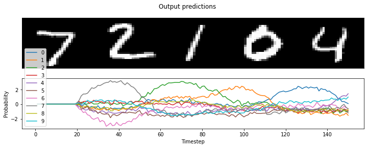
Our accuracy print-out is 100%, and we can also plot the results to see for ourselves:

# plot the neural activity of the convnet layers
plt.figure(figsize=(12, 4))

timesteps = loihi_sim.trange() / loihi_sim.dt

# plot the presented MNIST digits
plt.figure(figsize=(12, 4))
plt.subplot(2, 1, 1)
images = test_images.reshape(-1, 28, 28, 1)[:n_test]
ni, nj, nc = images[0].shape
allimage = np.zeros((ni, nj * n_test, nc), dtype=images.dtype)
for i, image in enumerate(images[:n_test]):
    allimage[:, i * nj : (i + 1) * nj] = image
if allimage.shape[-1] == 1:
    allimage = allimage[:, :, 0]
plt.imshow(allimage, aspect="auto", interpolation="none", cmap="gray")
plt.xticks([])
plt.yticks([])

# plot the network predictions
plt.subplot(2, 1, 2)
plt.plot(timesteps, loihi_sim.data[nengo_output])
plt.legend(["%d" % i for i in range(10)], loc="lower left")
plt.suptitle("Output predictions")
plt.xlabel("Timestep")
plt.ylabel("Probability")

Text(0, 0.5, 'Probability')

<Figure size 864x288 with 0 Axes>

Conclusions

In this example we’ve expanded on the process of converting a Keras model to an SNN with additional considerations that are important for SNN’s we want to implement on the Loihi. We then showed the additional steps required to prepare a network generated by the NengoDL Converter to run on Loihi, including modifying the input node and specifying the distribution of convnet layers across cores.