PES learning

In this example, we will use the PES learning rule to learn a communication channel.

import matplotlib.pyplot as plt

%matplotlib inline

import nengo
from nengo.processes import WhiteSignal
import nengo_loihi

nengo_loihi.set_defaults()

Creating the network in Nengo

When creating a nengo.Connection, you can specify a learning_rule_type. When using the nengo.PES learning rule type, the connection is modified such that it can accept input in its learning_rule attribute. That input is interpreted as an error signal that the PES rule attempts to minimize over time by adjusting decoders or connection weights.

with nengo.Network(label="PES learning") as model:
    # Randomly varying input signal
    stim = nengo.Node(WhiteSignal(60, high=5), size_out=1)

    # Connect pre to the input signal
    pre = nengo.Ensemble(100, dimensions=1)
    nengo.Connection(stim, pre)
    post = nengo.Ensemble(100, dimensions=1)

    # When connecting pre to post,
    # create the connection such that initially it will
    # always output 0. Usually this results in connection
    # weights that are also all 0.
    conn = nengo.Connection(
        pre,
        post,
        function=lambda x: [0],
        learning_rule_type=nengo.PES(learning_rate=2e-4),
    )

    # Calculate the error signal with another ensemble
    error = nengo.Ensemble(100, dimensions=1)

    # Error = actual - target = post - pre
    nengo.Connection(post, error)
    nengo.Connection(pre, error, transform=-1)

    # Connect the error into the learning rule
    nengo.Connection(error, conn.learning_rule)

    stim_p = nengo.Probe(stim)
    pre_p = nengo.Probe(pre, synapse=0.01)
    post_p = nengo.Probe(post, synapse=0.01)
    error_p = nengo.Probe(error, synapse=0.01)

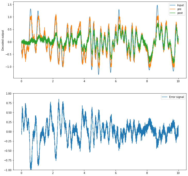
Running the network in Nengo

We can use Nengo to see the desired model output.

with nengo.Simulator(model) as sim:
    sim.run(10)
t = sim.trange()

0%

 

0%

 

def plot_decoded(t, data):
    plt.figure(figsize=(12, 12))
    plt.subplot(2, 1, 1)
    plt.plot(t, data[stim_p].T[0], label="Input")
    plt.plot(t, data[pre_p].T[0], label="pre")
    plt.plot(t, data[post_p].T[0], label="post")
    plt.ylabel("Decoded output")
    plt.legend(loc="best")
    plt.subplot(2, 1, 2)
    plt.plot(t, data[error_p])
    plt.ylim(-1, 1)
    plt.legend(("Error signal",), loc="best")


plot_decoded(t, sim.data)

While post initially only represents 0, over time it comes to more closely track the value represented in pre. The error signal also decreases gradually over time as the decoded values in pre and post get closer and closer.

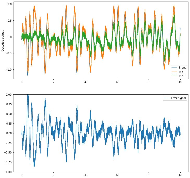
Running the network with NengoLoihi

with nengo_loihi.Simulator(model) as sim:
    sim.run(10)
t = sim.trange()

plot_decoded(t, sim.data)