2D Decision Integrator

This is a model of perceptual decision making using a two dimensional integrator. As mentioned in the book, the goal is to construct a simple model of perceptual decision making without being concerned with establishing how good or bad it is.

Rather than having two different integrators for each dimension, you will build the model using a single two dimensional integrator. This integrator can be used irrespective of the task demands since it effectively integrates in every direction simultaneously. This is neurally more efficient due to the reasons explained in the book.

# Setup the environment
import nengo
from nengo.processes import WhiteNoise
from nengo.dists import Uniform

Create the Model

The model has four ensembles: MT representing the motion area, LIP representing the lateral intraparietal area, input and output of the 2D integrator. The parameters used in the model are as described in the book. The 2D integrator resides in LIP. As discussed in the book an integrator requires two connections: here, the input from MT to LIP and the feedback connection from LIP to LIP.

Here, you will provide a an input of (-0.5, 0.5) to the model spanning over a period of 6 seconds to observe the model behaviour. In order to inject noise while the simulation runs, you can use the noise parameter when creating ensembles as shown. The reason for injecting noise is explained in the book.

# Create the network object to which we can add ensembles, connections, etc.
model = nengo.Network(label="2D Decision Integrator", seed=11)

with model:
    # Inputs
    input1 = nengo.Node(-0.5, label="Input 1")
    input2 = nengo.Node(0.5, label="Input 2")

    # Ensembles
    ens_inp = nengo.Ensemble(100, dimensions=2, label="Input")
    MT = nengo.Ensemble(100, dimensions=2, noise=WhiteNoise(dist=Uniform(-0.3, 0.3)))
    LIP = nengo.Ensemble(200, dimensions=2, noise=WhiteNoise(dist=Uniform(-0.3, 0.3)))
    ens_out = nengo.Ensemble(
        100,
        dimensions=2,
        intercepts=Uniform(0.3, 1),
        noise=WhiteNoise(dist=Uniform(-0.3, 0.3)),
        label="Output",
    )

    weight = 0.1
    # Connecting the input signal to the input ensemble
    nengo.Connection(input1, ens_inp[0], synapse=0.01)
    nengo.Connection(input2, ens_inp[1], synapse=0.01)

    # Providing input to MT ensemble
    nengo.Connection(ens_inp, MT, synapse=0.01)

    # Connecting MT ensemble to LIP ensemble
    nengo.Connection(MT, LIP, transform=weight, synapse=0.1)

    # Connecting LIP ensemble to itself
    nengo.Connection(LIP, LIP, synapse=0.1)

    # Connecting LIP population to output
    nengo.Connection(LIP, ens_out, synapse=0.01)

Run the Model

# Import the nengo_gui visualizer to run and visualize the model.
from nengo_gui.ipython import IPythonViz

IPythonViz(model, "ch8-2d-decision-integrator.py.cfg")

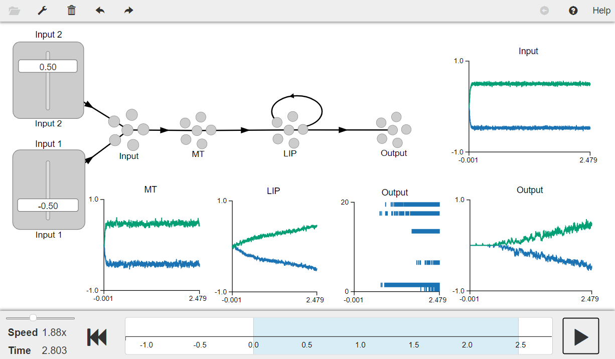
Press the play button in the visualizer to run the simulation. You should see the graphs as shown in the figure below.

The output plot on the bottom-right shows the output of the 2D decision integrator which is represented by a single two dimensional output ensemble. You can see that as MT encodes the input over time, LIP slowly moves towards the same direction as it acuumulates evidence that there is sustained motion in that direction.

Thus MT moves LIP in the right direction and once past a certain threshold, the output neurons start firing. To visualize this: 1) Select “spikes” from the right-click menu of the output ensemble. This will display a spike plot. 2) Run the simulation and then slide the blue box in the simulation control bar backwards. 3) You will see that the spikes become stronger once past a certain threshold (i.e., when LIP starts following MT)

from IPython.display import Image

Image(filename="ch8-2d-decision-integrator.png")